

What You’ll Learn ⚡
Grasp power quality fundamentals: voltage/frequency deviations, waveform distortion, and grid stability standards (IEC 61000‑4‑30 Class A)
Measure and interpret harmonics, interharmonics, total harmonic distortion (THD), total demand distortion (TDD), and grouped frequency bands up to 150 kHz
Analyze symmetrical components (positive, negative, and zero sequence) to assess system balance
Perform flicker and flicker emission analysis (Pst, Plt) per IEC 61000‑4‑15/‑21 and identify rapid voltage changes (RVC)
Set up DewesoftX’s Power Quality module: select channels, configure calculations, and use data displays like numeric, recorder, FFT/harmonic FFT, and waterfall plots
Capture raw data to study fault events and transient behavior while applying sensor compensation (amplitude/phase correction)
Export and visualize data in real-time or later—via built-in displays or external tools—ensuring compliance with power quality standards
Course overview
The Power Quality Analysis course provides a detailed examination of electrical power integrity and grid compliance using Dewesoft’s comprehensive hardware and DewesoftX software. It starts by defining power quality—covering waveform purity, voltage and frequency stability, and the impact of non‑ideal conditions on equipment and operations.
You’ll then explore key disturbances: from harmonics that distort ideal sinusoidal waves—up to the 3000th order and grouped per IEC 61000‑4‑7—to symmetrical component analysis for detecting unbalance, along with flicker and rapid voltage changes per IEC 61000‑4‑15 guidelines . The course also covers Total Demand Distortion (TDD), interharmonics, and frequency‑dependent groupings that allow deep examination of power quality dynamics up to high-frequency bands.
In hands-on modules, you’ll configure DewesoftX’s Power Quality module: selecting analog channels, choosing FFT vs. time-based calculations, and enabling inline sensor compensation to ensure high accuracy . You’ll engage in real-time monitoring using numeric displays, recorders, harmonic FFTs, waterfalls, and scope views—then learn how to record raw waveforms during fault conditions for detailed post-analysis.
Finally, the course teaches effective data management: exporting recorded data, applying calibration corrections, and generating visual reports that comply with industry standards. By completion, you’ll be able to deliver compliant power quality tests, troubleshoot disturbances, and integrate power quality modules into broader electrical diagnostics (including motor efficiency, power analysis, and PQ solutions across renewable, industrial, and grid applications).
What is power quality?
Power quality parameters describe the deviation of voltage from its ideal sinusoidal waveform at a given frequency. Such deviations can cause disturbances, outages, or damage to electrical equipment connected to the grid. It is essential to continuously monitor these parameters—starting in the development phase of electrical equipment, continuing through live operation, and beyond. For example, continuous monitoring at several points in the electrical grid helps to prevent and correct quality disturbances.
The Dewesoft Power Quality Analyzer measures all these parameters in accordance with the IEC 61000-4-30 Class A Standard. Compared to conventional power quality analyzers, it enables more detailed analysis, such as raw data storage, fault behavior evaluation, and the calculation of additional parameters.


The purpose of this chapter is to present all power quality parameters that Dewesoft can calculate. After a brief introduction and explanation of each parameter, the chapter provides a description of how the specific calculations are carried out and the variable names assigned to them in the DewesoftX software.
What are harmonics?
Harmonics are integer multiples of the fundamental frequency (e.g., 50 Hz for the grid in Europe) and cause distortion in the voltage and current waveforms. Harmonic voltages and currents, which result from non-sinusoidal loads, can affect the operation and lifespan of electrical equipment and devices. In motors and generators, harmonic frequencies can increase heating (iron and copper losses), affect torque (causing pulsations or reduction), create mechanical oscillations, and produce higher audible noise. They also accelerate the aging of shafts, insulation, and mechanical parts, ultimately reducing the overall efficiency of the motor.


The image illustrates such a case. In the first recording, the fundamental frequency is shown together with the 3rd, 5th, and 7th harmonic orders overlapping. So, what is the problem? After all, they are all sinusoidal waveforms with different amplitudes, right? Well, no. In the second recording, only the fundamental frequency is shown. This perfect sinusoidal waveform is the preferred signal for all electrical equipment, as it is the ideal form to work with.
The problem with harmonic orders is that they add to the fundamental frequency, creating non-sinusoidal waveforms. The subsequent recordings show how the sinusoidal waveform changes as more harmonic orders are introduced. It is clear that the higher the order, the less sinusoidal the wave becomes. By the 25th harmonic order, the waveform begins to resemble a square wave. The more higher-order harmonics are added, the squarer the waveform becomes. With infinitely many harmonics, the waveform would transform into a perfect square wave.
Overview
Current harmonics in transformers increase copper and stray flux losses, while voltage harmonics increase iron losses. These losses are directly proportional to frequency; therefore, higher-frequency harmonic components are more critical than lower-frequency ones. Harmonics can also cause vibrations and increased noise. The effects on other electrical equipment and devices are similar and typically include reduced efficiency and lifespan, increased heating, malfunctions, or even unpredictable behavior.


Dewesoft measures harmonics for voltage, current, and both active and reactive power up to the 3000th order. All calculations are implemented in accordance with IEC 61000-4-7 and can be selected in the power module, as shown in the following image. To calculate higher harmonics, the sampling rate must be adjusted accordingly. For example, at a sampling rate of 500 kS/sec or higher, DewesoftX can calculate up to the 3000th order.


Harmonics
Up to 500 harmonics can be calculated. In addition, there is an option to select all harmonics or only even or odd ones. If current channels are used in the power module, it is also possible to calculate phase angles, P, Q, and impedance.


Number of Sidebands
The basic idea of sidebands is that a certain frequency range is treated as one harmonic.
Example: One full sideband (±5 Hz) at a frequency of 50 Hz means that the range from 45 Hz to 55 Hz is considered the first harmonic. The same principle applies to all other harmonics. If two sidebands are selected, the first harmonic will cover the frequency range from 40 Hz to 60 Hz.


Number of Halfbands
According to IEC 61000-4-7 (page 22), the grouping of harmonic sidebands requires that only the square root of the quadratic half be added. This applies to the lowest and highest lines and is defined as halfbands in Dewesoft.
Example I: One sideband and one halfband at a frequency of 50 Hz means that the frequency range from 45 Hz to 55 Hz is considered the first harmonic. Additionally, the square root of the quadratic half of the 40 Hz and 60 Hz lines is included.
Example II: Two sidebands and one halfband at a frequency of 50 Hz means that the lines from 40 Hz to 60 Hz are taken with full amplitude, while the lines at 35 Hz and 65 Hz are included only with the square root of the quadratic half.


Interharmonics
Interharmonics include all frequency components that are not integer multiples of the fundamental frequency and are therefore not classified as harmonics.


Group FFT Lines
The higher-frequency components can be grouped into 200 Hz or 2 kHz bands, up to 150 kHz.
Depending on the measurement requirements, Dewesoft provides the option to select one or both of these harmonic groupings.


Full FFT
This option calculates a full FFT, which can then be exported to the database and displayed as a 2D graph.


Harmonics Smoothing Filter
This option enables the low-pass filter required by the IEC 61000-4-7 standard (page 23).
Background Harmonics
With this option, it is possible to subtract an existing and known harmonic pattern (magnitude and phase) from the measured values. This is typically applied during the commissioning of a high-power converter to determine the noise contribution of the converter.
This function is available for both voltage and current and can be selected from the Background Harmonics Editor in DewesoftX.
For this calculation, only the magnitude and phase angle of the harmonic pattern need to be entered, as illustrated in the input mask image below.


Example
The following images show a specific harmonic pattern measured using Dewesoft DAQ devices. A harmonic filter was then applied to the same measurement in DewesoftX, resulting in an adjusted harmonic pattern by subtracting the background harmonics.


How to perform a measurement with DewesoftX?
DewesoftX offers a range of display options for measurements such as voltage, current, active and reactive power, phase angle, impedance, interharmonics, and higher frequencies. These values can be shown as numeric displays, on recorders, or as 2D graphs, as illustrated in the following image. Users are free to configure the display as needed.


There are two options for displaying harmonics in DewesoftX: the Harmonic FFT and the 2D graph. The following image shows the icons used for these options—on the left is the Harmonic 2D graph, and on the right is the Harmonic FFT.


Harmonic FFT
In the Harmonic FFT, the harmonics of voltage, current, power, and reactive power can be displayed. The following image shows the voltage harmonics of a three-phase system.


2D Graph
With the 2D graph, voltages and currents of different phases can be displayed in a single graph. In addition, a wide range of display options is available, which the user can configure as needed for the specific application. The following figure shows the harmonics for the phase voltage of L1. On the right-hand side are the available display options for 2D graphs. Here, the graph type can be selected—either line or histogram—as well as the graph scale, which can be set to linear or logarithmic. The scaling of the graph axes can also be adjusted independently.


Persistence
There is also an option to display the persistence of the harmonics in the 2D graph. This means that when the harmonics change during a measurement, the variations appear blurred, as illustrated in the following figure.


Higher frequencies
Example: Higher frequencies from 2 Hz to 20 kHz displayed in a 2D graph as a histogram (application: HVDC converter station).


Interharmonics
Example: Interharmonics displayed in a 2D graph as a histogram. A peak appears at 900 Hz, which corresponds to the switching frequency of an HVDC converter operating in the public grid.


DewesoftX calculations
DewesoftX calculations for each harmonic/whole waveform


DewesoftX calculations for a 3 phase system


What is THD - total harmonic distortion?
The Total Harmonic Distortion (THD) of voltage and current can be calculated up to the 3000th order. In general, THD is defined as the ratio of the sum of all harmonic components to the fundamental frequency.


The most common sources of harmonics are loads controlled by converters such as diodes, thyristors, and transistors. The following images show a typical comparison of different light bulbs and the current waveforms (blue) they produce. The green waveforms represent the voltages. The corresponding values for voltage, current, THDI (Total Harmonic Distortion for current), power, and power factor for each light bulb are also shown.


How to calculate the total harmonic current (THC) and current total demand distortion (TDD)?
In addition to THD calculations, it is now possible to include THC and TDD calculations as well.
Total Harmonic Current (THC) represents the cumulative current from harmonic orders 2 to 40 that contribute to distortion in the current waveform. This value is particularly useful for determining the required specifications when installing modern active harmonic filters.
Current Total Demand Distortion (TDD) is defined as the ratio of the root-sum-square values of the harmonic currents to the maximum demand load current, multiplied by 100 to express the result as a percentage. The maximum demand load current can be defined in the software through an input field.
In the DewesoftX power module, under power quality, the THC and TDD options can be selected, as shown in the image below.


What are the symmetrical components?
Fundamental symmetrical components
Normally, an electric power system operates in a balanced three-phase sinusoidal steady-state mode. Disturbances, such as faults or short circuits, can lead to an unbalanced condition. As shown in the following image, the left-hand side depicts a balanced system with a symmetrical phase shift and equal vector distances, while the right-hand side illustrates an unbalanced system with an asymmetrical phase shift and uneven vector lengths.


By using the method of symmetrical components, any unbalanced three-phase system can be transformed into three separate sets of balanced components: positive, negative, and zero sequence.


The advantage of using a symmetrical balanced system is that calculations are simplified. If a fault occurs or a short circuit develops in the system, the unbalanced system can be transformed into a balanced system using symmetrical components. In this form, system calculations can be carried out with the standard formulas used for balanced systems. The calculated values are then transformed back into the unsymmetrical (real-world) phase voltages and currents. In general, a three-phase system can be represented and mathematically described as follows:


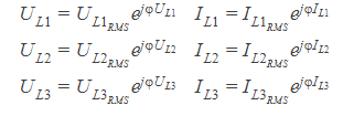
A balanced three-phase system, as shown in the image below, has the same RMS value for all line voltages and currents, with a 120° phase shift between each of them.


To explain the basic idea of symmetrical components, the first step is to define the operator as a unit vector with a phase angle of 120° (or 2π/32\pi/32π/3).
The voltages can be expressed mathematically in several ways, as shown in the table below:


Calculation of zero-sequence system
In a symmetrical system, the following equation is valid:
In a real system, the sum will not be zero. A voltage difference will occur, as shown in the following equation:
This voltage difference, divided by three, represents the so-called zero-sequence system:
The zero-sequence systems for the three phases (u10,u20,u30u_{10}, u_{20}, u_{30}u10,u20,u30) all have the same amplitude and phase. Therefore, only the value of the zero-sequence system U0U_0U0 is shown.
The calculation of the zero-sequence current is analogous to that of the voltage equation.
Calculation of positive-sequence system
The positive-sequence system has the same rotation direction as the original system (right). This means it will match the rotation direction of an electrical machine connected to the grid.
Since the values of the positive-sequence system for all three phases have the same amplitude (being symmetrical) and a phase shift of exactly 120°, it is sufficient to display only one value. In DewesoftX, this value is denoted as U1U_1U1.
Calculation of negative-sequence system
The negative-sequence system has the opposite rotation direction of the original system (left). This means it will rotate in the opposite direction of an electrical machine connected to the grid.
Since the values of the negative-sequence system for all three phases have the same amplitude (being symmetrical) and a phase shift of exactly 120°, it is sufficient to display only one value. In DewesoftX, this value is denoted as U2U_2U2.
Matrix of zero, positive and negative-sequence system
According to the following equations, the phase voltages and currents are transformed into symmetrical components. The result is three balanced three-phase systems: positive (U1,I1U_1, I_1U1,I1), negative (U2,I2U_2, I_2U2,I2), and zero-sequence (U0,I0U_0, I_0U0,I0).


As illustrated in the following images, an unbalanced system can be represented using the positive, negative, and zero symmetrical components. The image below shows an unsymmetrical system in a screenshot taken from DewesoftX.

")
The following image shows a screenshot of the three systems—positive, negative, and zero—of the symmetrical components in DewesoftX:

")
From the parameters of the symmetrical components (positive-, negative-, and zero-sequence), the original system can be easily reconstructed, e.g.:
The following variables are calculated in DewesoftX and represent the components of the zero- and negative-sequence systems in comparison to the positive-sequence system (for both the total and the fundamental harmonic).


Extended positive sequence parameters (according to IEC 614000)
The following calculations are based on Annex C of IEC 61400-21.
From the measured phase voltages and currents, the Fourier coefficients of the fundamental are calculated over one fundamental cycle TTT as the first step.
It is important to note that the index a refers to the line voltage L1L_1L1. The coefficients for L2L_2L2 (ubu_bub) and L3L_3L3 (ucu_cuc), as well as the coefficients for the currents (ia,ib,ici_a, i_b, i_cia,ib,ic), are calculated in the same way. Furthermore, f1f_1f1 is the frequency of the fundamental. The RMS value of the fundamental line voltage is:


Extended negative sequence parameters (according to IEC 614000)


Extended zero sequence parameters (according to IEC 614000)


What is a flicker?
Flicker refers to fluctuations (repetitive variations) in voltage. Flashing light bulbs are a clear indicator of high flicker exposure. Flicker is particularly common in grids with low short-circuit resistance and is caused by the frequent connection and disconnection of loads (e.g., heat pumps, rolling mills) that affect the voltage. A high level of flicker is perceived as psychologically disturbing and can be harmful to humans.


The Dewesoft Power Analyzer can measure all flicker parameters in accordance with the IEC 61000-4-15 standard. Flicker emission calculations are implemented according to the IEC 61400-21 standard and allow for the evaluation of flicker emissions fed into the grid by wind power plants and other power generation units.
The flicker-meter architecture is shown as a block diagram in the next image. It is divided into two parts: the simulation of the response of the lamp–eye–brain chain, and the online statistical analysis of the flicker signal, which produces the defined parameters. The blocks within the diagram will be discussed briefly.


Block 1
The first block contains a voltage-adapting circuit that scales the input mains voltage to an internal reference level. This method allows flicker measurements to be performed independently of the actual input voltage level and may be expressed as a percentage ratio.
Block 2
The second block recovers the voltage fluctuations by squaring the input voltage scaled to the reference level, thereby simulating the behavior of a lamp.
Block 3
The third block consists of a cascade of two filters, which may either precede or follow the selective filter circuit. The first low-pass filter removes the double mains frequency ripple components of the demodulated output.
The high-pass filter is then used to eliminate any DC voltage component. The second filter is a weighting filter that simulates the frequency response of the human visual system to sinusoidal voltage fluctuations of a coiled-filament, gas-filled lamp (60 W/230 V and/or 60 W/120 V).
Block 4
The fourth block consists of a squaring multiplier and a first-order low-pass filter. Human flicker perception—through the combined response of the eye and brain to voltage fluctuations applied to the reference lamp—is simulated by the nonlinear interaction of blocks 2, 3, and 4.
Block 5
The last block in the chain performs an online analysis of the flicker level, allowing direct calculation of key evaluation parameters.
The following image shows an example of a rectangular voltage flicker.


Measurement with DewesoftX: flicker
With DewesoftX, the Short-Term Perceptibility (Pst) and Long-Term Perceptibility (Plt) values can be calculated according to the IEC standard, using calculation times of 10 minutes and 120 minutes, respectively. The calculation time can also be adapted to the user’s needs by setting a calculation overlap and filter.


Flicker emission
Flicker emission (also called current flicker) refers to the proportion of flicker contributed to the grid by a producer or consumer. In addition, the internal voltage drop is calculated based on the grid impedance and the current flow.


The voltage drop is added vectorially to an idealized voltage source (U=Usim+R⋅I+L⋅didt)(U = U_{\text{sim}} + R \cdot I + L \cdot \tfrac{di}{dt})(U=Usim+R⋅I+L⋅dtdi). Using the flicker algorithm and this updated voltage, the current flicker values are then calculated.


Enable “Flicker” and “Flicker Emission”, then add the grid parameters. The short-circuit capacity and the grid impedance can also be specified. The phase corresponds to the grid impedance phase. Different phase angles can be entered as well (e.g., 30; 50; 70; 85).
The following table lists the channel names of the different parameters as they appear in the DewesoftX software. All parameters are calculated using the predefined methods of the IEC 61000-4-15 standard.


What are the rapid voltage changes?
Rapid Voltage Changes are parameters defined as a supplement to the flicker standard. They describe all voltage variations greater than 3% within a given time interval. These changes can then be analyzed using different parameters, such as the depth of the voltage change, duration, and steady-state deviation.
In DewesoftX, Rapid Voltage Change (RVC) calculations allow the determination of the maximum voltage drop (dmaxd_\text{max}dmax), the stationary deviation after the voltage drop (dcd_cdc), and the time at which the voltage falls below 3.3% of UnU_nUn. All values are calculated according to IEC 61000-4-15. Analysis can also be performed in compliance with IEC 61000-3-3 and IEC 61000-3-11. The following image shows the calculated parameters (IEC 61000-4-15, page 35).


Measurements with Dewesoft X
RVCs measurements with DewesoftX:


Steady-State Duration: This defines the duration of the steady state in seconds.
Hysteresis: This is the condition for the stationary deviation (du_dc), defined as a percentage (see IEC 61000-4-15, page 8).
Example: If a hysteresis of 0.2% and a steady-state duration of 1 s are defined, the stationary condition is reached when the voltage does not deviate by more than ±0.2% for 1 second.


How the channel list is defined in DewesoftX?
Dewesoft has developed a special FFT algorithm (software PLL) to determine the periodic time (frequency). The algorithm calculates the periodic time of the signal using this FFT method over a sampling window of multiple periods (typically 10 periods, configurable in the power module). The calculated frequency is highly accurate (in the millihertz range) and works reliably for all applications, including motors, inverters, and grids.
How Dewesoft X calculates the power of an AC system
While other power analyzers calculate power in the time domain, DewesoftX performs the calculation in the frequency domain. Using the predetermined period time, an FFT analysis of voltage and current is performed over a user-defined number of periods (typically 10 for electrical applications) and a configurable sampling rate. The FFT provides the amplitude of the voltage, current, and the cosine phi for each harmonic.
One major advantage of this FFT-based transformation is that the behavior of amplifiers and current or voltage transducers—in both amplitude and phase across the entire frequency range (using the Sensor XML)—can be corrected. This method of power analysis delivers the highest possible accuracy. Another advantage is that harmonic analysis and other power quality assessments can be carried out fully synchronized with the fundamental frequency.
With the FFT-corrected values, the RMS voltages and currents are calculated from the RMS values of each harmonic.
The rectified mean is the average of a rectified signal. For an AC signal, it represents the average of the absolute values of voltage or current.
The rectified mean is used, for example, in transformer testing, as it is proportional to the magnetic flux.
The power values for each harmonic, as well as the total values, are calculated using the following formulas:


Where the power quality can be applied?

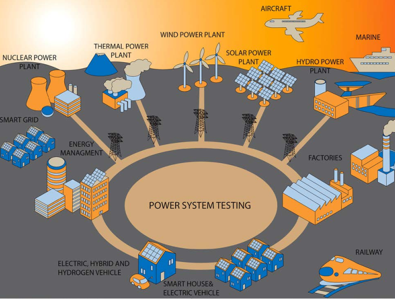
Power grid
fault and transient recording
power quality analysis (IEEE 1159, EN50160)
Transformer
efficiency analysis (IEC 60076-1)
no-load and short circuit testing
vibration, noise
Wind, solar and CHP
power performance (IEC 61400-12)
power quality (IEC 61400-21 / FGW-TR3)
active and reactive power (FGW-TR3)
behavior at faults (FGW-TR3)
Nuclear power plant
turbine and generator
testing rod drop
castor testing
Turbine and generator
modal analysis
order tracking
balancing
rotational vibration
efficiency measurement
Smart grid and energy management
power system testing
load profile
demand-side management
Aircraft
power system testing
fault and transient recording
hybrid testing
harmonics analysis
Marine
power system testing
fault and transient recording
hybrid testing
Railway
power system testing (AC and DC rails)
power quality analysis
fault and transient recording
short-circuit analysis
pantograph and current shoe testing
E-mobility
electric two-wheeler
electric vehicle
hybrid vehicle (series and parallel)
hydrogen vehicle
Equipment testing
fans and pumps testing
circuit breaker testing
filter analysis
harmonics analysis according to IEC 61000-3-2/-12
voltage changes according to IEC 61000-3-3/-11
CE conformity of electrical devices (harmonics, flicker) and a lot more
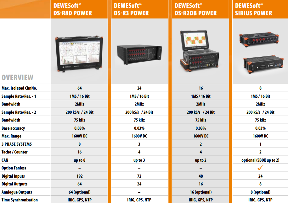
Dewesoft's power Instruments


Page 1 of 14