

What You’ll Learn 🎯
Configure DewesoftX Orbit Analysis: setup frequency source, RPM, calculation, runout compensation, reference orbit, and machine geometry
Connect and calibrate proximity probes (X/Y) and keyphasor/tacho sensors for journal-bearing orbit measurement
Capture and analyse raw, filtered, averaged orbits, polar and Bode plots, shaft centerline trajectories, waterfalls, and clearance circles
Apply runout compensation to remove shaft irregularities and set reference orbits for comparative analysis
Identify and interpret common rotor faults: imbalance, misalignment, oil whirl, oil whip, resonance effects
Use X-Y plots and polar diagrams to assess bearing lubrication state, rotor dynamics, and clearance behavior
Monitor journal bearing condition over time and across speed ranges (runup, steadystate, coastdown)
Export reports and integrate orbit data with other modules like FFT, Order Tracking, rotor balancing, and historical databases
Course overview
The Orbit Analysis course enables engineers and vibration analysts to master rotor dynamics diagnostics using DewesoftX and compatible DAQ hardware. By measuring the shaft’s motion within journal bearings—via dual proximity probes and a tacho/keyphasor—the course teaches how to visualise rotor orbits as raw, averaged, or filtered plots alongside polar and Bode representations.
You’ll gain practical experience configuring measurement parameters: selecting RPM range, harmonic orders, FFT resolutions, and enabling runout compensation and reference orbits. The course guides you through detecting common fault conditions—such as imbalance, misalignments, subsynchronous vibrations like oil whirl/whip, or resonance—using dedicated widgets like clearance circles and waterfall spectrograms.
Additionally, the training covers real-time monitoring across machine operation phases (runup, steadystate, coastdown), report generation, and integration with other Dewesoft modules like Order Tracking, FFT, rotor balancing, OPC UA, and Historian logging . By the end, attendees are equipped to deploy orbit analysis in R&D or operational environments, enhancing predictive maintenance and reducing downtime in turbomachinery applications.
View the Orbit Analysis webinar
Introduction to orbit analysis
Why should you use orbit analysis?
Steady, continuous operation with minimal malfunctions and vibrations is essential for maximizing productivity and ensuring the reliable performance of a machine—whether it is a large rotating mass in a power plant or a high-revving compressor. By understanding rotor movement, various phenomena related to lubrication and bearing conditions can be identified, allowing machine operations to be optimized.
To achieve this, the measurement and analysis of rotational vibration data are crucial. Dewesoft Orbit Analysis is an ideal tool for examining rotor dynamic behavior, assessing any motion restrictions that cause vibration, and preventing potential damage to rotating machinery. Such damage can lead to premature wear of components and, ultimately, critical failure.
Orbit Analysis enables continuous monitoring and evaluation of the current condition of journal bearings and how they have performed over time during operation.
It is specifically designed for these bearing types to inspect and diagnose shaft or journal movement, oil lubrication behavior, and clearance levels.

Dedicated display widgets for orbit analysis help provide a clear overview of the condition of one or multiple bearings. Such analysis is crucial for understanding the impact of lubrication oil, shaft load, rotational speed, clearance, and bearing wear.
When should you use orbit analysis?
Orbit analysis is suitable for the evaluation of journal bearings. These bearings are also sometimes referred to as bushings, plain bearings, or sleeve bearings. All of these types feature a fluid lubrication layer between the shaft and the bearing, allowing the shaft to slide with some freedom of movement within the clearance.
Orbit analysis is not applicable to roller bearings, gears, or other bearing types that involve rolling action or a direct connection between the shaft and the bearing. This is because there is no fluid medium or lubrication layer between the components, and therefore no loose shaft movement. Instead, for such direct-contact bearings and gears, Order analysis is the appropriate method of evaluation.
What is needed to configure and get going with orbit analysis?
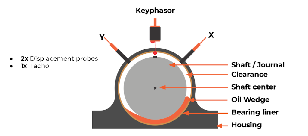
The basic measurement setup for orbit analysis consists of the following:
pair of proximity probes (also called eddy-current probes) per bearing,
a keyphasor (3rd proximity probe or a tacho sensor),
a data acquisition system,
orbit analysis software,
and a computer.
By detecting shaft proximity in two directions (X and Y), rotor movement can be calculated and displayed throughout the measurement.
Orbit analysis system configuration
The Dewesoft Orbit Analysis system is highly flexible and can be configured for single or multiple bearing measurements simultaneously. The number of input channels can be expanded at any time. The DAQ system can also be configured to support various sensor connections concurrently—including thermocouples, RTDs, IEPE/ICP® accelerometers, strain gauges, and more.
A typical Orbit Analysis measurement system typically consists of the following elements:
SIRIUSi isolated data acquisition system with 8xLV signal amplifiers or 6xLV-2xLV+ (additional two counter) amplifiers.
2-8x Eddy-current probes
DewesoftX Orbit Analysis option
Optional:
FFT Analyzer option
Order tracking analysis option
Rotor balancing option
OPC UA Client/Server option
Historian time-series database
MODBUS protocol option


Industry case examples
Orbit analysis is one of the main diagnostics tools for rotating machinery using journal bearings, such as turbomachinery. Turbomachinery provides kinetic energy to operations enabling movement - a function that is widely used in industrial processes to move solids, liquids, or gases through drivers, driven components, and transmissions such as:
Compressors
Drills
Generators
Turbines
Engines
Pumps
Blowers


Such rotating machinery as shown above is applied in a variety of industries, e.g. automotive, chemical, oil and gas, metals, HVAC or mining, and in the majority of different power plants:
Hydroelectric
Nuclear
Thermal
Gas
Coal
Biomass
Below is an example that shows how a journal bearing is monitored at a hydropower plant. By monitoring the shaft centerline position together with both orbit plots, polar plots, shaft speed, and much more, it is possible for the operator to follow the bearing condition, both regarding bearing wear and tear, but also regarding e.g. lubrication oil conditions.


Proximity probe
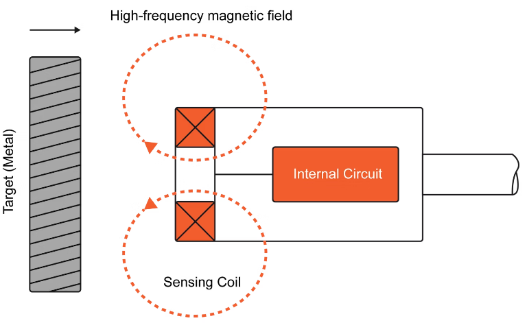
A proximity sensor can detect a nearby object without making physical contact and then output a pulse or voltage signal. There are several types of proximity sensors, selected based on the composition of the object(s) to be detected.


For example, an inductive proximity sensor generates an electromagnetic field around its sensing end. According to the well-known magneto-resistive effect, the resistance of certain materials—particularly ferrous ones—changes when exposed to magnetic fields. Most proximity sensors take advantage of this effect by generating a small magnetic field and detecting when it is significantly altered or interrupted by the presence of such materials.
When a sensor is placed near a rotating shaft and a ferrous feature is affixed to the shaft—positioned to pass close to the sensor with each revolution—it becomes a highly reliable and accurate speed sensor. The sensor detects interruptions in the magnetic field and outputs a pulse or voltage signal that any DAQ system can display and record.

Capacitive proximity sensors can also detect non-metallic objects using the principle of capacitive coupling. Instead of generating an electromagnetic field, they produce an electrostatic field. When an object enters this field, it alters the capacitance in the sensor’s oscillator circuit. The sensor detects this change and generates an output signal. For both magnetic and capacitive proximity sensors, the sensitivity to the target object can be adjusted.
Proximity sensor pros:
Very reliable because they never make contact with the objects being detected. Wear and tear are virtually non-existent
Very low initial and operating cost
Capacitive types can also be used to measure the thickness
Inductive types are not affected by water, mud, etc.
Proximity sensor cons
Limited detection distances - most inductive sensors are limited to 70mm (2.76 in.)
They require external power
Analog in setup - proximity probes
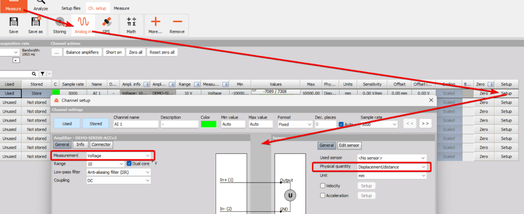
In the Analog In setup, the channels must be configured for the use of proximity probes.
Typically, the configuration for each bearing includes three eddy-current probes: Y, X, and Keyphasor.
Depending on whether the eddy-current probes use a separate signal conditioner or are connected directly to the input on Dewesoft hardware, different amplifiers are used.
In both cases, Voltage mode is selected under Measurement, and Displacement/Distance is chosen as the physical quantity.

Orbit analysis setup - frequency channel setup
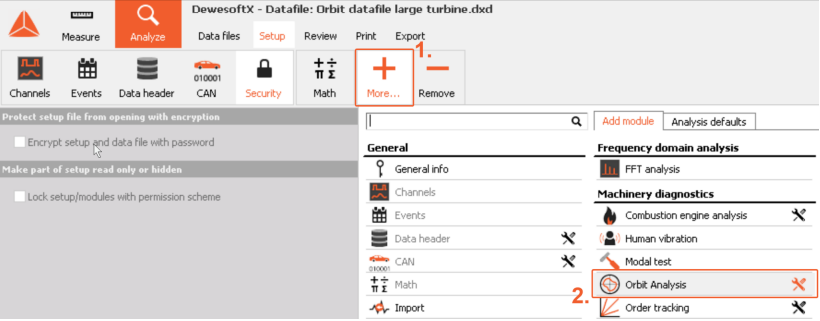
The Orbit Analysis module can be added to a setup by clicking the “+ More” button, where various application modules are available.
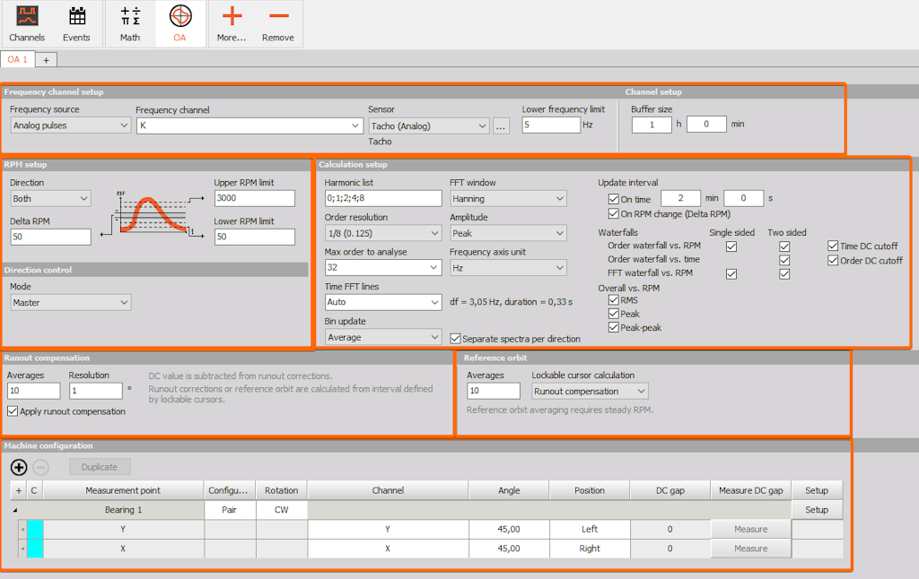
When the module is added, the following setup screen appears:
Frequency channel setup
RPM setup
Calculation setup
Runout compensation
Reference orbit
Machine configuration

Frequency channel setup
To determine engine rotation speed, a frequency source must be configured. For Orbit Analysis, a third proximity probe—also called a keyphasor—is most commonly used, as it detects a flat or wedged section on the shaft. This detection generates the necessary pulse per revolution, from which the operating speed is determined.
To provide flexible configuration options, the Orbit Analysis module supports several different sensor types that can be selected as the frequency source:

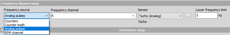
Counters
For Orbit Analysis, multiple pulses or transient spikes per revolution are often used. This means that a Tacho (digital) input is typically selected for such applications when using sensors that are connected and configured as counters.

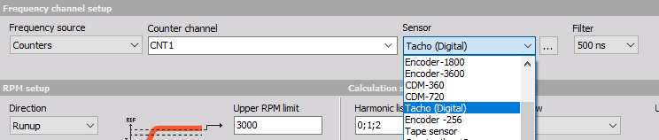
To support a wide range of configuration options, various additional counter sensors are available in the dropdown menu, including multiple encoders and CDM sensors. In addition, different filter settings can be applied to the selected frequency source signals.
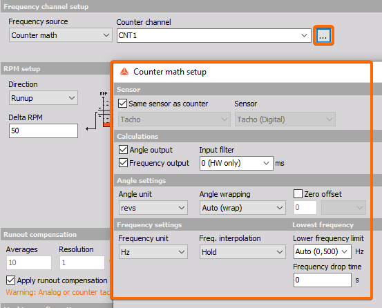
Counter math
With the Counter Math module, it is possible to determine and recalculate counter angle and frequency outputs both during live measurements (online) and during data file analysis after the measurement (offline).
This can be useful, for example, when correcting a faulty counter setting that wasn’t identified during the measurement, or when fine-tuning a setting to see if it produces better results.
Counter Math supports features such as frequency smoothing, tooth size adjustment, software filtering, and angle wrapping.
If the results from Counter Math are better for your specific data file, you can use the math output as input for other modules that work with counters, such as Orbit Analysis, Order Tracking, or Torsional Vibration.

Analog pulses
When the frequency source is set to Analog Pulses, an analog time channel must be selected. Various sensors that generate analog pulses are supported.

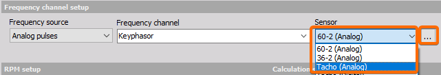
Tacho(Analog): 1 pulse per revolution using a proximity probe or a similar type of analog sensor
36-2 (Analog) or 60-2 (Analog): sensor with 58 or 34 teeth and two missing teeth
To configure the selected analog sensor, click the three-dot icon to open the Angle Sensor Math setup.
In the Angle Sensor Math setup, additional settings are available for configuring the sensor:

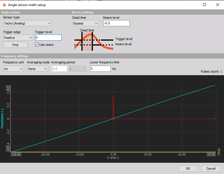
Trigger edge
Trigger level (can also be found automatically by selecting ‘’Find’’),
Retrigger level,
Retrigger time,
Output channel unit (Hz or RPM) and
Averaging
a preview of analog tacho signals and triggers.
The lowest detectable frequency limit can be defined in the user input field. The system will not detect frequencies lower than the specified value.
RPM channel
In addition to analog and digital sensors, any signal or channel that directly represents RPM (e.g., 0–10 V corresponds to 0–4500 RPM) can be used as a frequency source. However, since this option does not contain zero-angle information, phase extraction is not possible.
Orbit analysis setup - RPM setup
In the RPM setup section, the lower and upper RPM limits are defined, along with the Delta RPM width and the test direction.

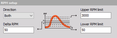
To configure the analysis according to the test conditions of the specific rotating machinery during measurement—and to capture all necessary data—the RPM setup section includes essential settings related to test direction, operating speed range, and the density of value calculations during the test run.
Direction
Orbit Analysis supports the measurement of various machine operating scenarios. Whether you need to measure only runup, coastdown, or both, the analysis can be easily configured via a dedicated dropdown menu.
Since turbomachinery often operates for extended periods in steady-state conditions between runup and coastdown, selecting Both in the dropdown will automatically add a third operating condition: Steady-State. Each direction generates a dedicated set of channels for displaying measured data, which can be shown either on separate widgets or combined into a single widget for comparison.
Delta RPM
Delta RPM defines the speed change interval at which data is updated during measurement for the speed channel and all Orbit Analysis output channels that include speed-related information. These include: Filtered Orbit (e.g., Orbit H1), Shaft Centerline, Polar Plot, Order Waterfall vs. RPM, and FFT Waterfall vs. RPM.
Lower and upper RPM limits
Upper and lower RPM limits define the calculation range and are used to correctly configure the resampling algorithm, depending on the maximum order to be extracted. These limits should be set according to the expected speed range of the machine being measured:
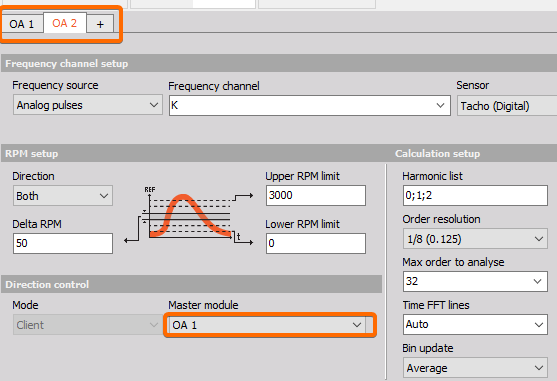
Direction control
This makes it possible to control the Direction setting under Measure for multiple Orbit Analysis modules simultaneously. In setups where multiple Orbit Analysis modules are added and the Direction is set to Both, you can choose to link the direction control across modules, instead of changing the direction for each one individually.
The Mode parameter can be set to either Master or Client. For Client modules, you must select the Master module to which they should be linked.
For example, if module OA1 is the Master and module OA2 is a Client linked to OA1, then these two modules are connected. Any direction change made under Measure in one module will automatically apply to the other as well.

Orbit analysis setup - calculation setup
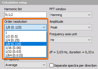
Harmonic list
Filtered orbit extraction is configured by entering the desired order numbers in the Harmonic List field, separating each entry with a semicolon (;). In the example below, the first, second, and third harmonic orbits are extracted.

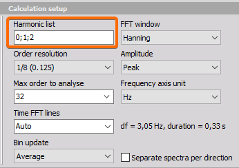
Order resolution
The selected order resolution defines the step size in the order waterfall between individual extracted orders. The higher the resolution, the greater the number of lines between the orders.

In an FFT, if the line resolution is 0.5 Hz, the required data window must be 2 seconds. The same principle applies to order resolution: if the resolution is set to 0.25 orders, 4 revolutions are required for one data block. The higher the desired order resolution, the more slowly the RPM must change.
Maximum order to analyze
Depending on the measurement application, the maximum order to be analyzed must be set high enough to capture all relevant orders. If, for example, higher-order components are not required in the analysis, a lower value can be selected from the dropdown. This will reduce the necessary sample rate and decrease the amount of data stored.
Time FFT lines
This setting affects the FFT cascade output. A higher number of lines results in better resolution but also increases CPU load. It supports Auto, predefined values selected from a dropdown, or a user-defined custom number of lines.
Bin update
Bin update defines how the output data for each RPM speed bin is calculated.
Always - When multiple values or spectra belong to the same bin, then the newest bin values will overwrite previous values and the newest values will be used in the output for that bin.
First time - When multiple values or spectra belong to the same bin, then only the first bin values will be used in the output for that bin.
Average - When multiple values or spectra belong to the same bin, then averaging for the values and individual and spectral lines will be performed over all values belonging to that bin.
Maximum - When multiple values or spectra belong to the same bin, then the maximum value for all values and individual spectral lines across all spectra belonging to that bin will be kept.
FFT window
Different windows are available for the FFT:
Rectangular,
Hanning,
Hamming,
Flat top,
Triangle,
Blackman (selected by default),
Exponential down and
Blackman - Harris.
Amplitude
Depending on the selected amplitude in the dropdown, the following scaling is applied to the Bode and Polar plots: Peak, RMS, and Peak-to-Peak.
Frequency axis unit
The frequency axis unit for the FFT Waterfall vs. RPM can be selected from the dropdown list.
Separate spectra per direction
Enabling Separate Spectra per Direction will create the selected spectral channels under each direction’s channel group. When disabled, the spectral results are combined across all directions.
Update interval
The update interval defines the criteria by which data—such as speed, shaft centerline, and polar plots—are updated during the measurement.
There are two different criteria for updating the data:
On RPM change (Delta RPM) - data is updated each time a defined Delta RPM value is exceeded. This is usually selected if the measurement consists of runup or coastdown or both.
On time - Values are updated on a defined time interval, regardless of the Delta RPM specified. This update criterion is suitable for steady-state operating conditions when RPM change criteria are not going to be triggered. Both update criteria can be selected at the same time to appropriately cover different operating conditions.
Orbit analysis waterfalls
The Orbit Analysis module supports Order Waterfall spectrograms versus RPM and versus time, as well as FFT Waterfall versus RPM.
These can be easily enabled by ticking the checkbox in the Ch. Setup section. The results are displayed using the 3D Graph widget, which is further explained in the Measurement & Visualisation section.
Spectra versus RPM can be created as either single-sided or two-sided. Single-sided spectra have an order or frequency axis starting from 0, while two-sided spectra have an axis centered around 0.
Two-sided spectra are particularly useful when analyzing the phase difference between X and Y bearing sensors.
Overall vs. RPM
Overall vs. RPM results are 2D arrays showing overall displacement levels across the defined RPM speed range. These results provide a clear overview and can be useful for documenting critical speed intervals that should be avoided.
Orbit analysis setup - runout compensation
Runout compensation is used to remove shaft irregularities from the measured values during analysis. In the Ch. Setup, the user defines the desired RPM at which the compensation will be performed, along with the number of averages (revolutions) to include in the calculation and the desired angle resolution.

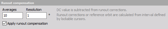
Under Measure, the Orbit Analysis module provides a display template specifically designed for runout compensation measurements. When the Runout Start button is pressed, the measurement begins, and the number of averages starts counting up.
Runout compensation values are calculated in the angle domain, which means you can perform runout compensation measurements even while operating at variable speeds.
Orbit analysis setup - reference orbit
The reference orbit is a valuable tool for easily comparing current operating conditions to those from a previous measurement.
During the measurement, the reference orbit can be quickly acquired through a dedicated measurement screen.
The number of averages included in the measurement is defined by the user in the Averages field.

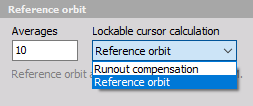
Averages - specifies how many times the deflections at individual angles are averaged together.
Lockable cursor calculation - Used when calculating runout compensations and reference orbits in Analyze mode (post-processing). Set this parameter to the desired calculation type to use the correct lockable cursors.
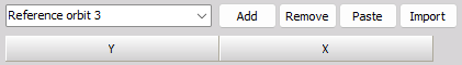
After measuring reference orbits, the determined values can be displayed in the Bearing Setup section by pressing the Paste button. The data will be added to the selected reference orbit table:

Orbit analysis setup - machine configuration
Any number of bearings can be defined within the machine train using Dewesoft OA. The machine configuration setup can then be further divided into subsections:

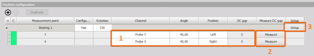
1 - Quick settings
2 - DC gap
3 - Bearing setup
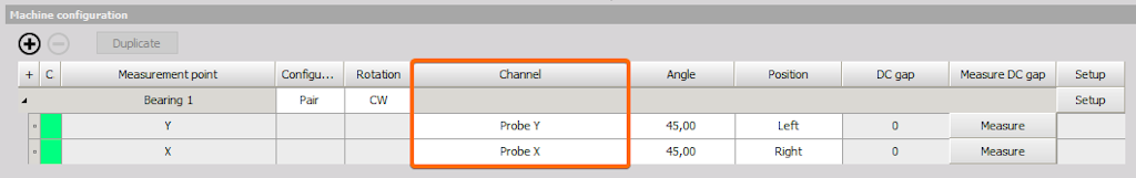
Quick settings
Under the Channel section, the appropriate input channels must be assigned as X and Y probes for each individual bearing.

Next, configure the angles and positions at which the probes are mounted.

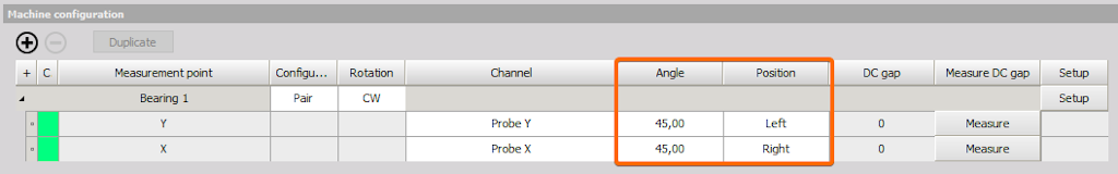
To make the configuration of the Angle and position easier, the graphical representation is available upon entering the Bearing setup
DC gap
Most of the time when proximity probes are mounted, there will be a certain DC component present. Dewesoft Orbit Analysis supports easy measurement of the DC gap by clicking on the Measure button next to the individual probe.

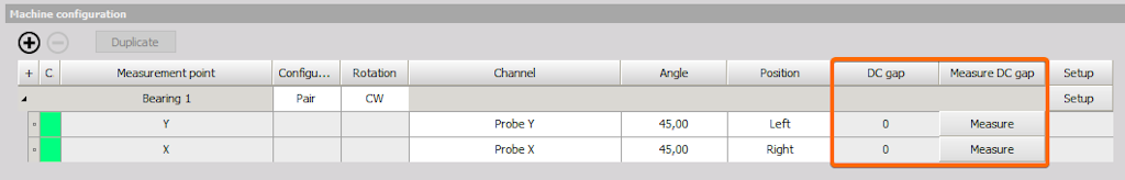
To simplify the configuration of angle and position, a graphical representation becomes available when entering the Bearing Setup.
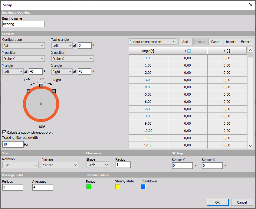
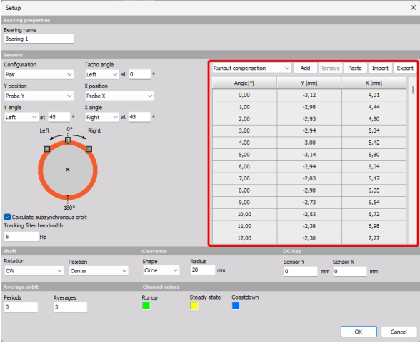
Bearing setup
Upon selecting Setup under Machine Configuration, a dedicated Bearing Setup window opens, containing all the advanced options for configuring the bearing settings:
sensor configuration,
subsynchronous orbit extraction,
shaft and clearance circle configuration,
average orbit definition, and
DC gap manual input.
Within this setup window, the user defines both the runout compensation and the reference orbit.

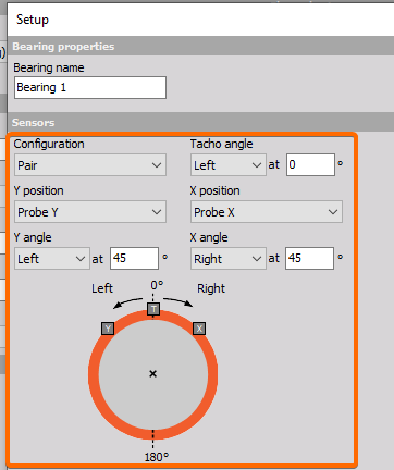
Bearing properties
Under Bearing Name, the user can enter a unique name to easily identify the corresponding component.
Sensor
The graphical representation of the shaft—along with direction and angle—helps ensure the correct configuration of sensor settings.
In this section, the user selects the configuration:
Pair is selected when two probes per bearing are used and
Mono in case only one is used.
In addition to selecting the configuration, the correct probe channels must be assigned to the Y and X positions, and their angle and direction must also be set.
The same applies to the Keyphasor under the Tacho angle setting.

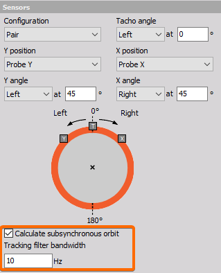
Dewesoft Orbit Analysis supports the extraction of subsynchronous orbits, which can be used to detect fluid-induced instabilities such as whirl and whip. The calculation of the subsynchronous orbit is enabled via a dedicated checkbox, and the tracking filter bandwidth is defined in the corresponding input field:

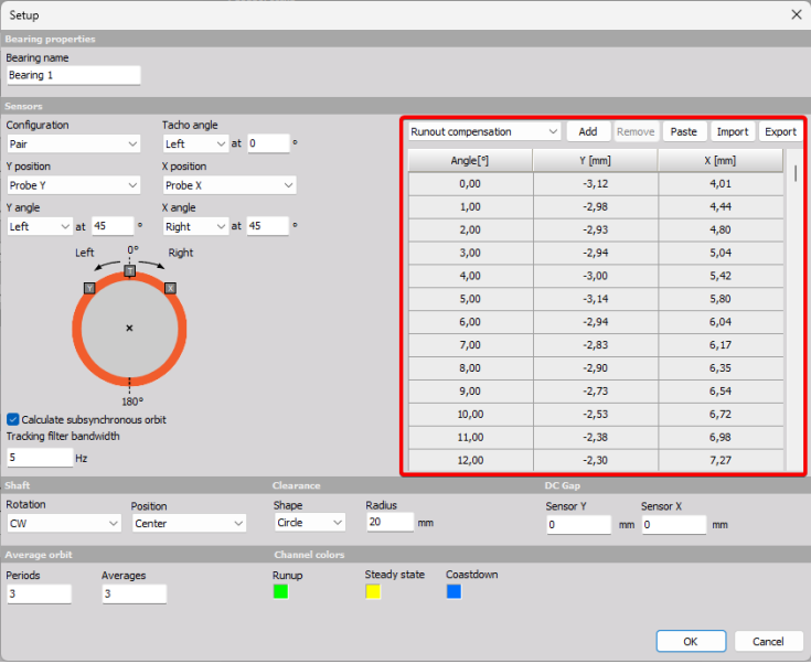
Runout compensation
Runout compensation is necessary whenever shaft shape irregularities are present, as they could be misinterpreted as actual movement during measurement. Dewesoft OA supports multiple methods for establishing runout compensation:
1.) Paste - allows the user to paste values for runout compensation from previous measurements. The angle step needs to be defined the same in the Ch. setup as it was for the data that will be pasted and the data structure of the columns needs to be as stated below in the Import paragraph.
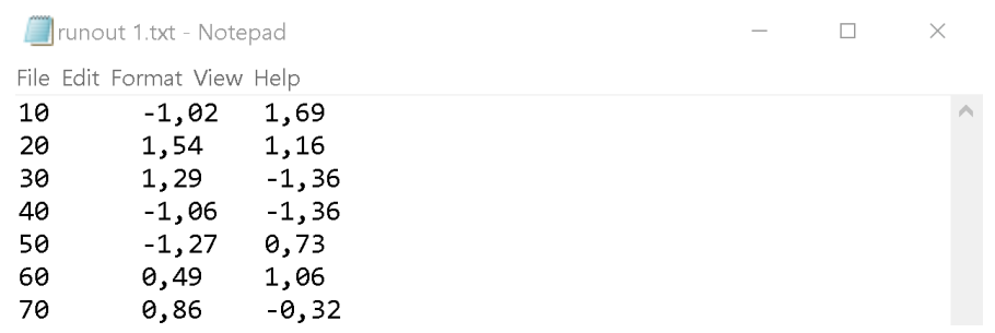
2.) Import - allows import of .txt files containing the runout compensation data. The data structure is important as it needs to contain an angle in the first column, a Y value in the second, and X in the third. A good way to achieve correct structure is to input it in separate columns in Microsoft Excel and then save it as a .txt file. Example .txt file is seen below:

3.) Measure - The last and perhaps most important way of determining the runout compensation is to measure it directly with Dewesoft. This is also the easiest way of doing it as it requires a single click operation in Measure and calculated values are automatically stored in the Ch. setup.
Shaft
This section of the channel setup is dedicated to configuring shaft-related settings. The direction of shaft rotation is selected from the Rotation dropdown menu. The dropdown allows the user to choose between CW (clockwise) and CCW (counterclockwise) rotation.

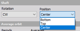
The Position dropdown defines the shaft's starting position relative to the bearing diameter.
Clearance
Dewesoft Orbit Analysis allows for straightforward definition of the clearance circle under the Clearance section of the Machine Configuration Setup.
Users can choose between circular and elliptical shapes for the clearance area and use the input fields to enter the radius (for a circle) or width and height (for an ellipse).

Average orbit
The average orbit can be configured to display more than a single revolution at a time. This is defined by the value entered in the Periods field—e.g., setting it to 5 means the average orbit will display 5 revolutions.
The user also defines how many revolutions to average by entering the desired number in the Averages input field.
DC gap
In addition to measuring and automatically compensating for the DC gap, Dewesoft Orbit Analysis also allows users to manually enter DC gap values.
This is especially useful for large turbines, such as those found in power plants, where completely static conditions (0 RPM) are rarely achieved. In such cases, the DC gap is measured during probe installation and manually entered for use in later measurements.
Reporting
Monitoring and alarms
Data output streaming to 3rd party system
Report generation
Orbit analysis output channels
The Orbit Analysis module includes a wide variety of result types, many of which generate multiple output channels. A complete list of these results—along with brief descriptions, the number of channels created per type, and the recommended display widgets for visualization—is provided in the table below:
| Function type | Description | Number of channels | Display widget |
|---|---|---|---|
| Orbit [X] X | [X] order orbit showing displacement in two directions | Per bearing, per order | Orbit plot |
| r[X]+ | Positive-sided component of [X] order | Per bearing, per order | Digital meter |
| r[X]- | Negative sided component of [X] order | Per bearing, per order | Digital meter |
| G[X] | [X] order orbit ellipse semi-major axis, a | Per bearing, per order | Digital meter |
| K[X] | [X] order orbit ellipse semi-minor axis, b | Per bearing, per order | Digital meter |
| Shaft center | Bearing shaft center displacement | Per bearing, per direction | Orbit plot |
| Raw orbit | Orbit with all orders over time | Per bearing | Recorder, scope |
| Bearing [X] Raw orbit | Orbit with all orders over time, with angle info for bearing [X] | Per bearing | Orbit plot |
| Average orbit | Orbit with all orders averaged over a number of blocks | Per bearing | Orbit plot, 2D graph |
| Bearing [X] waveform | Waveform with all orders of probe X or Y over time or revolutions | Per bearing, per probe | Orbit waveform |
| Subsynchronous orbit | Oil whirl/whip orbit | Per bearing | Orbit plot |
| Subsynchronous order | Oil whirl/whip variable fractional order number | Per bearing | Digital meter |
| DC gap | Probe DC gap over time | Per bearing, per probe | Digital meter |
| Time [X]X | [X] order data over time | Per bearing, per probe, per order | Recorder, digital meter |
| Polar [X]X | [X] order data with RPM stamps | Per bearing, per direction, per probe, and per order | Polar plot |
| Order waterfall vs. speed [two-sided] | Two-sided order spectra across the RPM speed range | Per bearing, per direction*, and per probe | 3D graph |
| Order waterfall vs. time [two-sided] | Two-sided order spectra over time | Per bearing, per direction*, and per probe | 2D graph, 3D graph |
| FFT waterfall vs. speed [two-sided] | Two-sided FFT spectra across the RPM speed range | Per bearing, per direction*, and per probe | 3D graph |
| Order waterfall vs. speed | Order spectra across the RPM speed range | Per bearing, per direction*, and per probe | 3D graph |
| FFT waterfall vs. speed | FFT spectra across the RPM speed range | Per bearing, per direction*, and per probe | 3D graph |
| Bode plot [X]X | [X] order bode showing magnitude and phase vs. RPM speed | Per bearing, per direction*, and per probe | 2D graph |
| Overall RMS | Total RMS value across the RPM speed range | Per bearing, per direction*, and per probe | 2D graph |
| Overall peak | Total peak value across the RPM speed range | Per bearing, per direction*, and per probe | 2D graph |
| Overall peal-peak | Total pk-pk value across the RPM speed range | Per bearing, per direction*, and per probe | 2D graph |
| SPP Average orbit SPPy | Average orbit longest y direction pk-pk displacement | Per bearing | Digital meter |
| SPP Average orbit SPPx | Average orbit longest x direction pk-pk displacement | Per bearing | Digital meter |
| SPP Average orbit SPPmax | Average orbit longest overall pk-pk displacement | Per bearing | Digital meter |
| SPP Raw orbit SPPy | Raw orbit longest y direction pk-pk displacement | Per bearing | Recorder, digital meter |
| SPP Raw orbit SPPx | Raw orbit longest x direction pk-pk displacement | Per bearing | Recorder, digital meter |
| SPP Raw orbit SPPmax | Raw orbit longest overall pk-pk displacement | Per bearing | Recorder, digital meter |
| SPP orbit [X]X SPPy | [X] order orbit longest y direction pk-pk displacement | Per bearing, per order | Digital meter |
| SPP orbit [X]X SPPx | [X] order orbit longest x direction pk-pk displacement | Per bearing, per order | Digital meter |
| SPP orbit [X]X SPPmax | [X] order orbit longest overall pk-pk displacement | Per bearing, per order | Digital meter |
| Speed | Speed RPM for the OA instance | 1 | Digital meter |
| Direction | Test direction for the OA instance | 1 | Input control, Discrete display |
Visualization - orbit plot
Each bearing with assigned channels added to the machine train will automatically generate a dedicated predefined display. This display includes a set of Orbit plots, Polar plots, and 2D graphs, as well as a digital meter for speed and an input control dropdown for selecting different operating conditions—if Both is selected under the RPM setup.
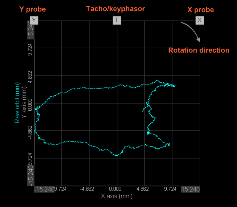
Orbit plot
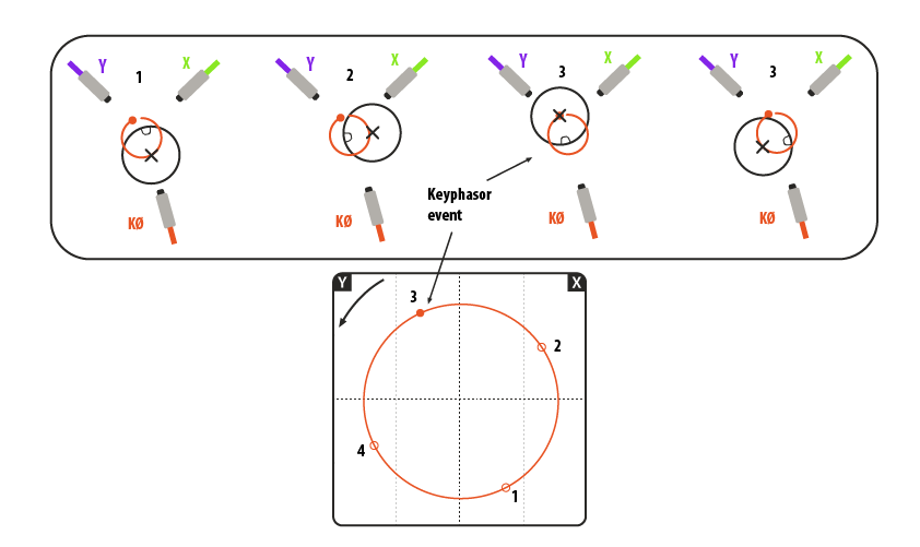
The Orbit Plot is a dedicated widget for the Orbit Analysis module. It displays data from two time-domain channels, creating a two-dimensional visual representation of the motion of a rotating shaft.
The widget graphically shows the position of the proximity probes, along with the tacho (keyphasor) position and the direction of rotation.
Various output channels available in the Orbit Analysis module can be displayed on the Orbit Plot:
Raw orbit,
Average orbit,
Filtered orbit (e.g. Orbit H1, Orbit H1, …),
Subsynchronous orbit and
Shaft centerline

When the Orbit Plot widget is selected, a settings tab appears on the left side of the Measure display, allowing the user to configure the axis.

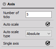
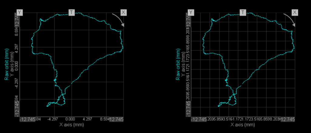
Number of ticks - changing the number of ticks will increase them on the Orbit plot accordingly. The left picture below shows 5 ticks and the right picture shows 15 ticks:

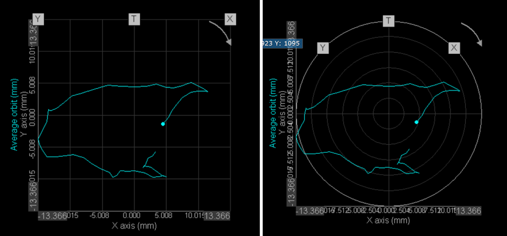
Auto scale - ticking the checkbox will automatically scale the axes of the Orbit plot. There are two different Auto scale types: Absolute and Relative.
Absolute auto-scale always keeps the zero in the center of the plot and therefore gives a better indication of orbit size and position relative to the center of the bearing:

Relative auto-scale sizes the axes according to the maximum current dimension of the measured orbit. This makes the orbit shape easier to observe and acts as a sort of zoom. The zero in this case is not always in the center position:

Single axis - this checkbox determines the behavior of how channel names are shown next to the orbit plot when showing multiple channels on the same graph. In the below example, two harmonic orbits are shown on the same orbit plot. The left image shows a single axis switched on and the right image shows a single axis switched off:

In addition to axis configuration, various Drawing Options are available when the Orbit Plot widget is selected:

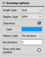
Graph type - The user can select either Grid or Circle. The difference between the two graph types is shown below - the left image shows a Grid and the right image shows a Circle:

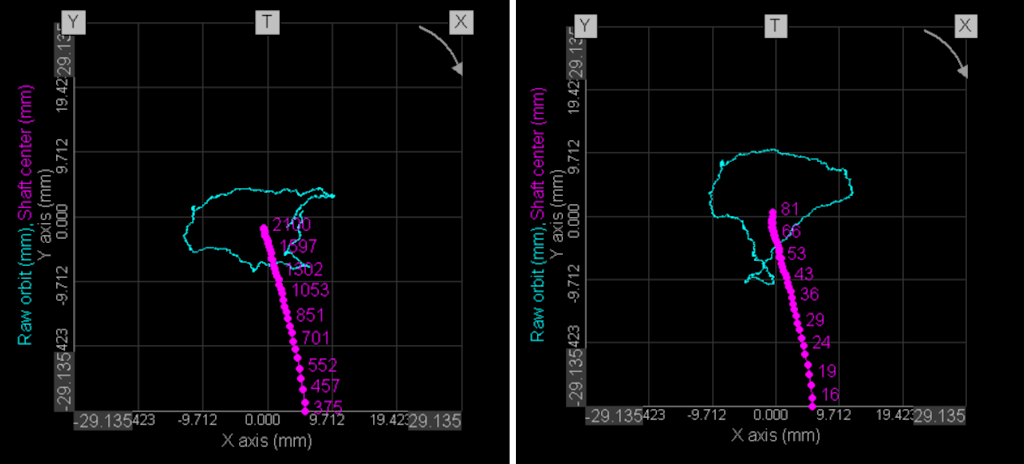
Display type - The user has the option to select either RPM or Time (in seconds) to be displayed when the Shaft center is assigned to the Orbit plot. The below images show the difference, the left image displays RPM and the right image displays Time together with the shaft center points:

The images below illustrate the relationship between the probe locations and the shaft position. The Orbit Plot widget demonstrates how four different positions are plotted. In Location 1, the black shaft is farther from the proximity probes than in Location 3:

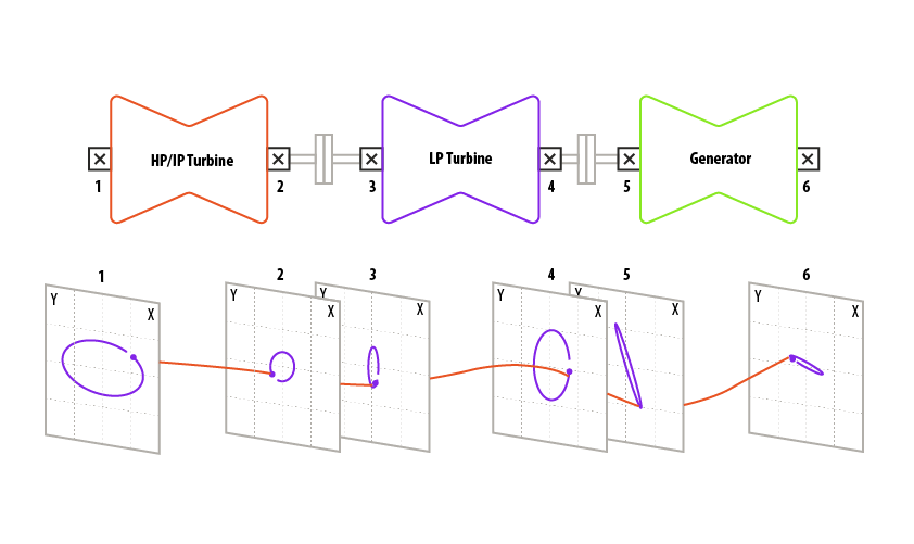
In the picture below, six orbit plots are shown for six different bearings. This helps illustrate the relationship between keyphasor dot positions across bearing locations, and in turn, provides a better understanding of the rotor shaft's deflection shape.
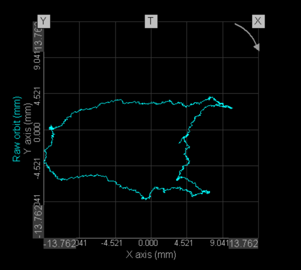
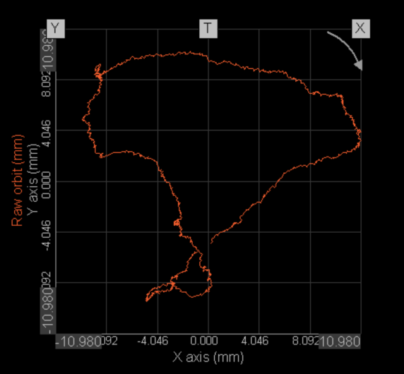
Visualization - raw orbit
The raw orbit, also called the direct orbit, plots scaled time-domain data directly from a pair of orthogonal probes mounted at the same axial position on the rotating machine.
The raw orbit channel group can be displayed on the Orbit Plot.

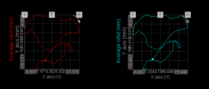
Visualization - average orbit
The 2D Graph widget supports both multi-trace and multi-graph display modes, allowing the average orbit to be visualized in either format.
Average orbits from different bearings can also be displayed on the Orbit Plot using multi-graph mode.
Below is an example of average orbits from two bearings positioned closely along the shaft length, shown in multi-graph mode on the Orbit Plot:

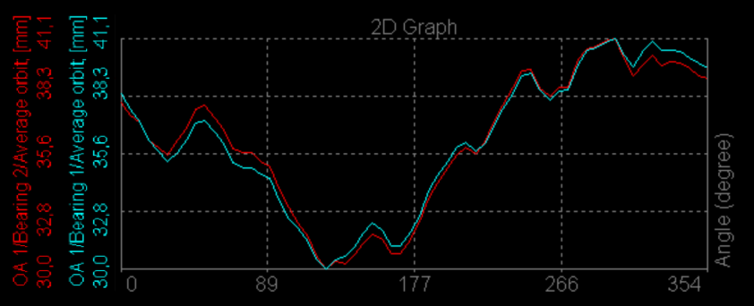
Average orbits from two bearings positioned close to each other along the shaft length, displayed in multi-trace mode on the 2D Graph:

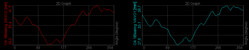
Average orbits from two bearings positioned close to each other along the shaft length, displayed in multi-graph mode on the 2D Graph:

Visualization - filtered orbit
The filtered orbit, also called the harmonic orbit, represents the extracted orbit of the order specified by the user in the Harmonic List section of the Calculation Setup.
For each harmonic entered in the list, a separate channel is created:

Each created filtered orbit channel can be displayed on the Orbit Plot widget. As with raw and average orbits, the filtered orbit can be shown in both multi-trace and multi-graph modes.
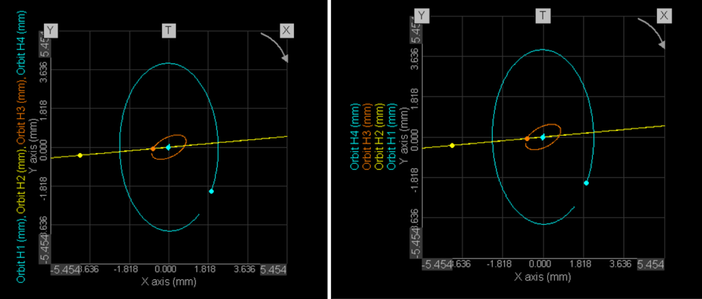
Filtered orbits H1–H4 displayed in multi-trace mode on the Orbit Plot:

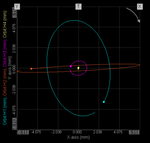
Filtered orbits H1–H4 displayed in multi-graph mode on the Orbit Plot:


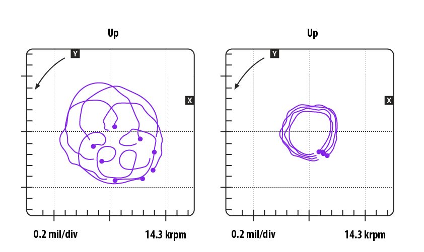
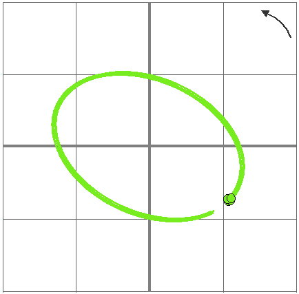
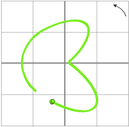
Examples of 1X and subsynchronous orbits
The orbit on the left shows subsynchronous fluid-induced instability. Note the multiple keyphasor dots, as the frequency is not a fraction of the running speed.
The orbit on the right is predominantly 1X. The keyphasor dots appear in a tight cluster, indicating dominant 1X behavior.
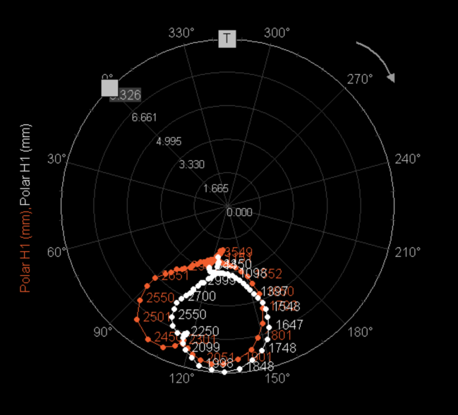
Visualization - polar plot
The Polar Plot is a dedicated widget featured in the Dewesoft Orbit Analysis module. It enables the simultaneous representation of amplitude, phase, and speed, along with the shaft center, on a single display—providing a comprehensive overview of machine operation in one widget.
Each probe has a corresponding set of Polar Plots for each extracted order of the filtered (harmonic) orbit. Polar Plots for runup, coastdown, and steady-state conditions are written into separate channels, depending on the selection in the Input Control dropdown, output channels, and visual representation.
The predefined Orbit Analysis measurement display includes a Polar Plot widget for each probe used per bearing. When using Orbit Analysis with a pair of probes, a pair of Polar Plots is automatically generated, with each plot representing data from one of the probes—Y and X.

Visualization - orbit waveform graph
The Orbit Waveform Graph widget plots displacement data from the X and Y bearing sensors over a user-defined time duration or a specific number of revolutions.
Each new tacho keyphasor crossing is marked with a dot on the graph, as illustrated below:

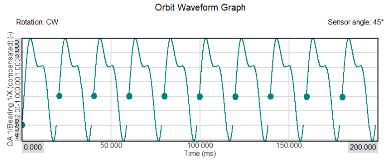
When a fixed time duration is selected, the number of revolutions varies over time, as illustrated above.
You can select a fixed time duration by setting the History Type parameter to Time. Then, specify the desired duration using the Display Time setting in the graph.
If History Type is set to Revolutions, you can choose the number of revolutions you want to display.

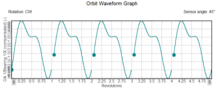
When the History Type is set to Revolutions, you can choose to display the axis with either a fixed revolution count or angle, or with a varying time length that changes as the rotational speed changes—ensuring the number of plotted revolutions remains constant.
Typical display for orbit analysis
Over the years of Orbit Analysis development, a set of display layout designs has been created that are typical for this application. With Dewesoft’s advanced customization capabilities, it is easy to create, edit, and modify these standard display layouts in just a few clicks.
The following sections provide examples of how to generate such display layout templates.
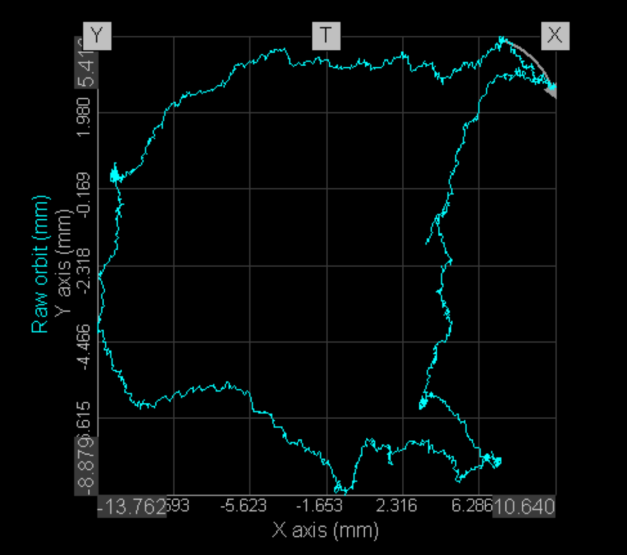
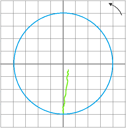
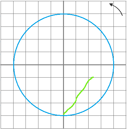
Raw orbit with clearance circle
This view is created by assigning the Raw Orbit channel group to the Orbit Plot widget and enabling the clearance circle option in the widget settings on the left side. The clearance circle must be defined in advance within the Orbit Analysis channel setup.

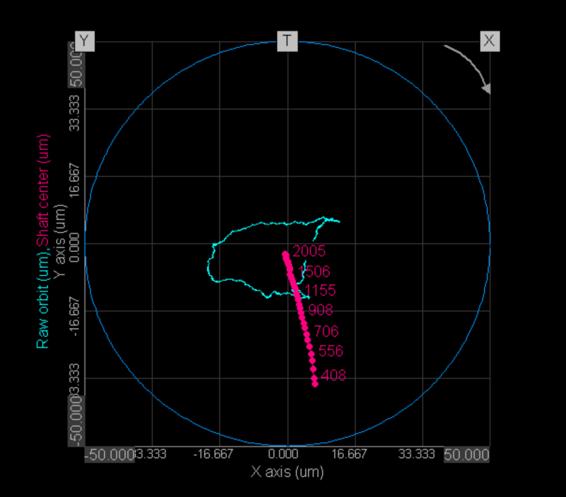
Full motion graph
This view is created from the Raw Orbit with a Clearance Circle by adding the Shaft Center channel to the Orbit Plot. In other words, it is generated by assigning both the Raw Orbit and Shaft Center to the Polar Plot widget and enabling the Clearance Circle option.
The clearance circle must be defined in advance within the Orbit Analysis channel setup.

Runout compensation display
Runout compensation, sometimes called slow-roll compensation, is applied to correct for any shaft irregularities—such as flattenings or other variations in diameter along the circumference—that would otherwise be detected by the proximity probes along with the actual shaft movement.
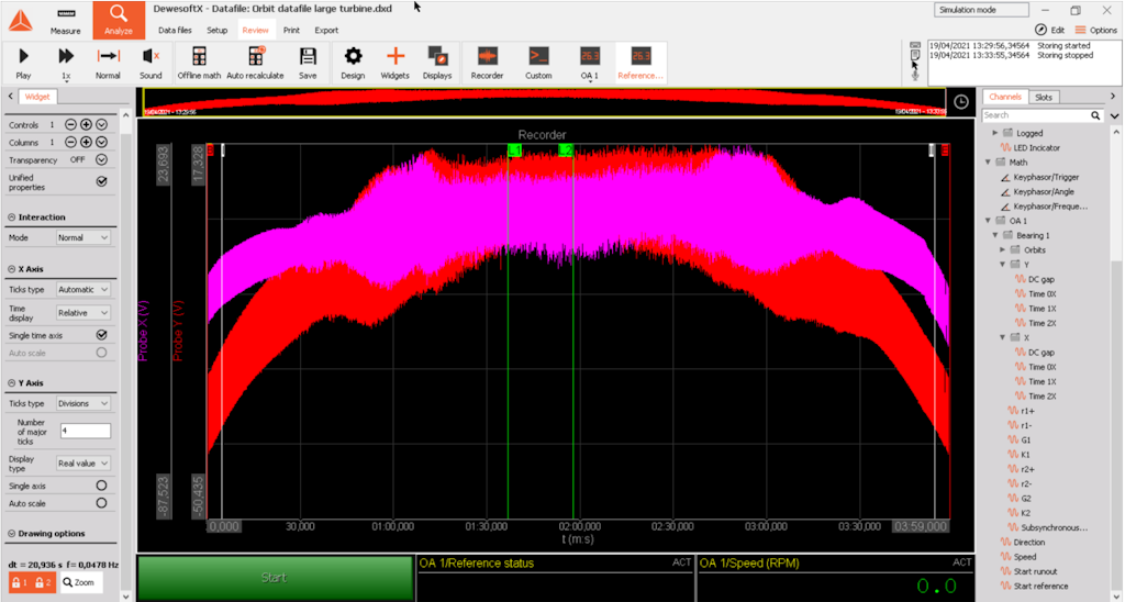
Once configured in the Ch. Setup, the compensation is performed through a dedicated measurement display, which is automatically generated along with predefined overviews for each bearing and a Reference Orbit display.

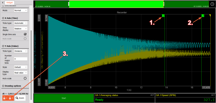
The predefined Runout Compensation display consists of the following elements:
1. Recorder with raw signals from proximity probes
2. Start button to initiate the runout compensation
3. Measurement status
4. Current speed of the machine

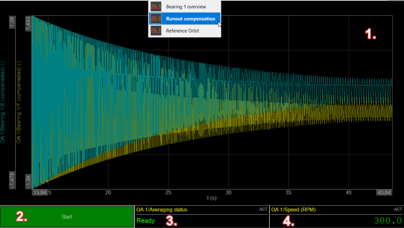
When the measurement begins, the status in the measurement status bar changes from Ready to displaying the progress of the measurement. The process collects the number of averages defined by the user in the Ch. Setup section under Runout Compensation.


The system displays the status Done after the runout compensation measurement has been successfully completed:


After the Runout Compensation measurement is marked as Done, the calculated values are automatically added to the setup and can be viewed in the Ch. Setup, under the Machine Configuration → Bearing Setup page:

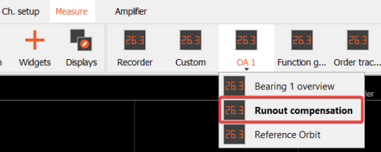
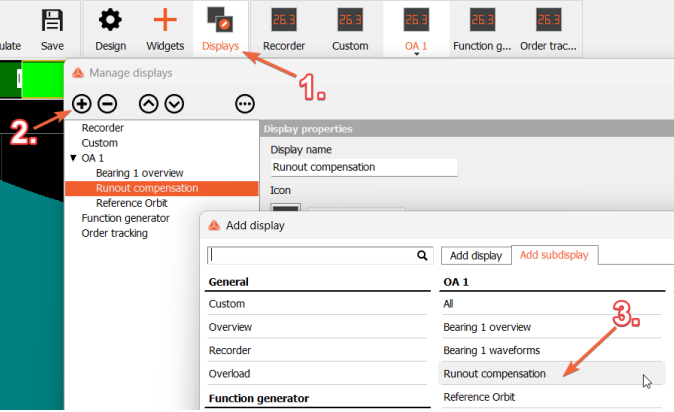
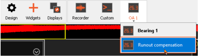
If the Runout Compensation display needs to be added manually, follow these steps:
1. Select Displays
2. Select + the button
3. (Optionally) Go to the Add sub-display tab
4. Select Runout compensation


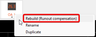
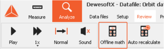
Recalculation of stored data
Orbit analysis can be recalculated using the raw signals from the proximity probes and the frequency source that were stored during the measurement. To recalculate the data, simply open the data file containing the raw signals and, in Analyze mode, navigate to Offline Math:

1. When in Setup, add the Orbit Analysis by selecting More… and choosing Orbit Analysis from the list of modules:

2. Having added the Orbit Analysis module, configure it by following the same steps described in the previous sections.
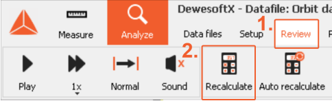
3. Return to Review and select Recalculate

4. The recalculated output channels are now displayed on the predefined display.

Recalculating runout correction
Along with all output channels from Orbit Analysis, runout compensation can also be recalculated during post-processing using the raw data from the proximity probes.
To recalculate and apply runout compensation in Analyze mode, follow the steps below:
1. Navigate to the Runout compensation sub-display template.

2. In the Runout compensation display, place the two cursors over the section of raw data you wish to use for the runout compensation and lock them.

3. Click on Recalculate to determine the runout compensation data:

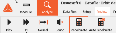
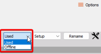
If you see the Offline Math button instead of the Recalculate button, first set the Orbit Analysis module to Offline under Setup.
4. After Recalculation, the calculated values are automatically added to the setup and can be seen under the Machine configuration - Bearing Setup page:

Recalculating reference orbit
Using the acquired raw data, it is also possible to define the reference orbit in Analyze mode. To recalculate and store the reference orbit in Analyze mode, follow the steps below:
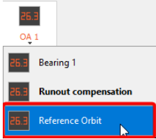
1. Navigate to the pre-defined Reference orbit sub-display template:

2. Place the two cursors over the desired region from which you wish to acquire data to define the Reference orbit, and then lock the cursors:

3. Select Recalculate. If you see an Offline math button instead of the Recalculate button then set the Orbit analysis module to Offline first under Setup.
4. Now the newly calculated Reference orbit data are copied to the clipboard and can be pasted directly into a Reference orbit data table found under the Bearing Setup page.
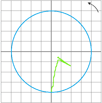
Machine fault - normal operation
Normal operation is characterized by acceptable vibration levels at all measurement positions. Critical speeds may be excited during speed transients, but the vibration amplitude remains within acceptable limits. Trend plots show consistent amplitude with little or no variation under different loads. The dominant vibration frequency is 1X, with minimal or no vibration at other frequencies.
Amplitude trend
The amplitude trend plot shows a consistent amplitude with no significant dependence on load or time.
1X phase trend
The 1X phase trend will display a constant phase value over time.
Waveform
Direct waveform plots show no truncation, no frequencies other than 1X, and no spikes.
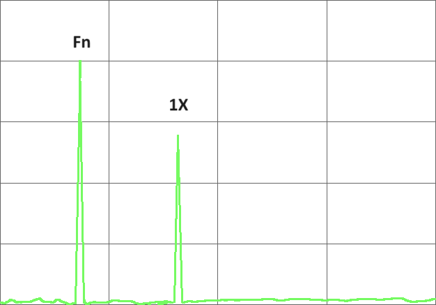
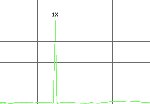
Spectrum

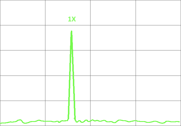
The half-spectrum plot shows a single dominant peak at the 1X frequency, with no significant vibration at other frequencies.
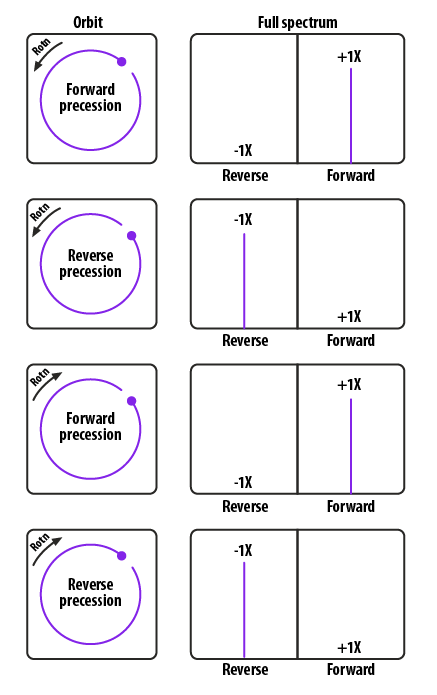
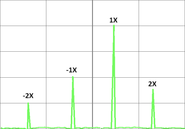
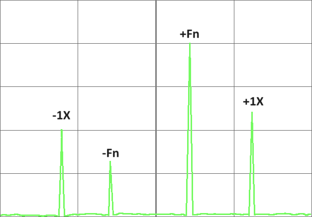
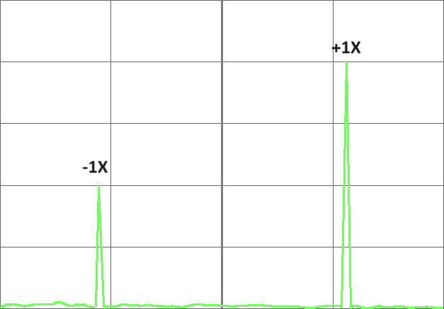
Full spectrum / Two-sided spectrum

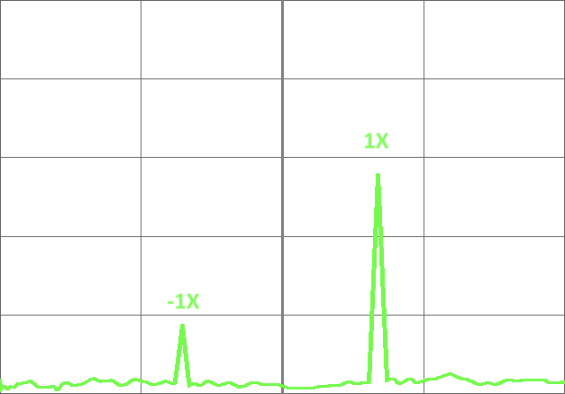
The full-spectrum plot shows a single dominant positive peak at the +1X frequency, with no significant vibration at other frequencies. The peak at –1X is lower than the peak at +1X.

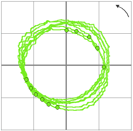
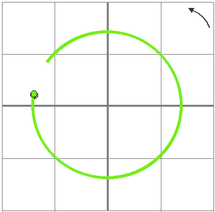
Direct orbit

A circular or slightly elliptical orbit with no evidence of truncation or loops is observed. The phase trigger indicates forward precession.
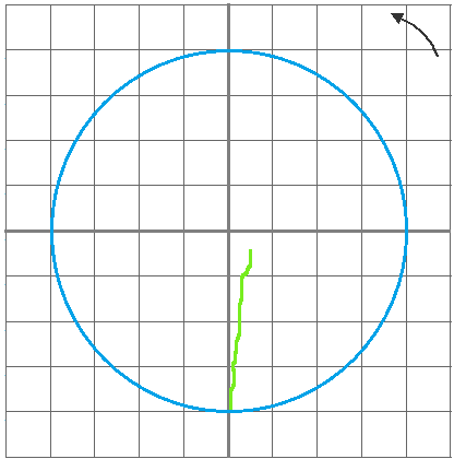
Shaft centerline

The shaft centerline plot shows a normal path from zero to full speed, with no sudden changes. Eccentricity remains below the vertical centerline at full speed.
Bode plot amplitude

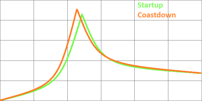
The Bode plot (amplitude) shows acceptable amplitude at the critical speed. Some variation between startup and coastdown responses is typical.
Bode plot - phase
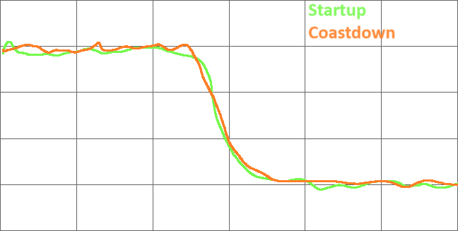
The Bode plot (phase) shows a smooth phase shift across the typical speed range, with the rate of change matching previous runup or coastdown events. The phase at both full speed and very low speed remains consistent between events.
Polar plot

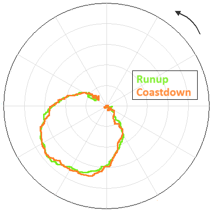
The polar plot shows similar amplitude at low speed, through the critical speed, and at full speed across transient events, with acceptable maximum amplitudes at both the critical speed and full speed.
Waterfall
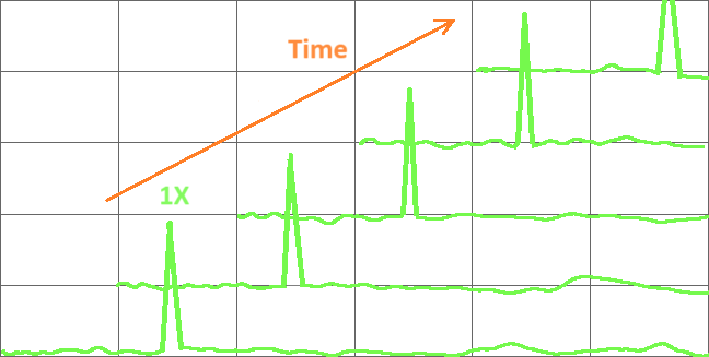
The waterfall plot shows a fairly constant amplitude across multiple periods, with no significant variation in the 1X amplitude.
Other operational symptoms
Bearing temperature trends remain constant with changes in speed and load, staying below alarm limits. Audible noise near the machine shows no changes compared to previous surveys and no signs of abnormal rattling.
Machine fault - mechanical imbalance (blade loss)
A sudden imbalance may be caused by blade loss, the loss of a balance weight, or another component that is normally attached to the rotor. This may occur during normal operation or during a load or speed transient. It can be distinguished from an electrically induced imbalance because the changes in vibration characteristics (amplitude/phase) are not reversible by altering the load or speed.
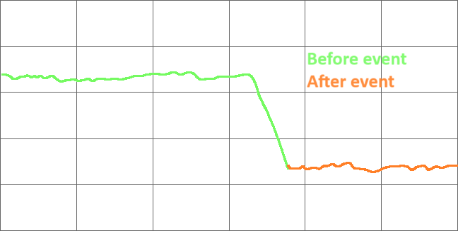
Amplitude trend
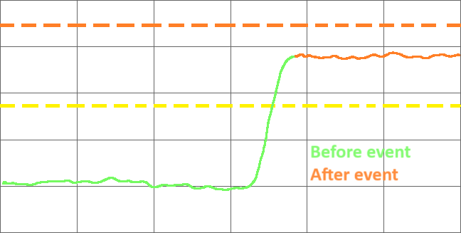
Vibration amplitude trends show a sudden increase in amplitude. Similar step changes may also be observed in vibration phase trends.
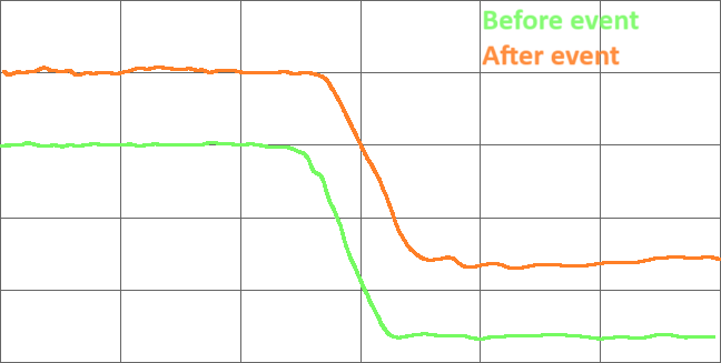
1X phase trend
The 1X phase trend will exhibit a step change. The phase may increase or decrease depending on the angle between the location of the lost material and the residual unbalance vector.
Waveform
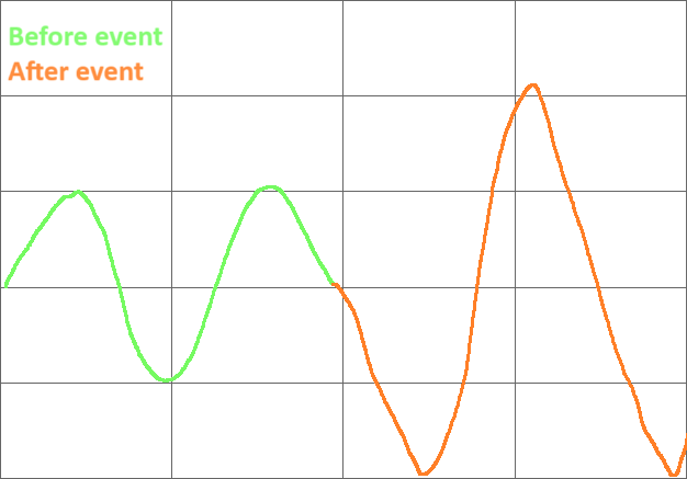
The direct waveform plot at the time of damage will show a sudden increase in amplitude. If the amplitude is excessive, some truncation may occur.
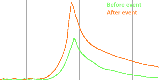
Spectrum
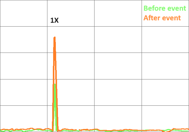
After the event, the half-spectrum will show an increase in 1X amplitude compared to the values before the event. Some small-amplitude peaks at n–X frequencies may also be present.
Full spectrum / Two-sided spectrum
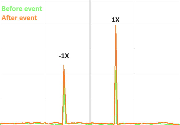
The full-spectrum plot will show an increase in both +1X and –1X peaks. There may also be an increase at ±nX frequencies. The +1X peak will be higher than the –1X peak unless another fault is present.
The direction of shaft precession is indicated by a dominant line in the “CCW” or “CW” component.
• How flat the ellipse will be is determined by the relative size of CCW and CW components
• When the orbit is circular there is only one spectrum line
• When the orbit is a line the CCW and CW spectrum components are equal
• The smaller the difference between components, the more elliptical the orbit.

Direct orbit

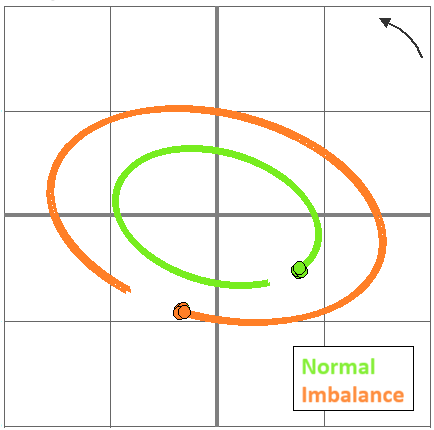
The direct orbit plot will show an increase in amplitude, as well as a phase change before and after the event—indicated by a shift in the position of the phase trigger marker.
Shaft centerline

The shaft centerline plot will typically show a sudden jump in position immediately after the event, followed by a return to near the pre-event position shortly thereafter.
Bode plot - amplitude
The Bode plot (amplitude) will show an increase in amplitude at all speeds following a blade loss. The critical speed will remain unchanged, and the amplification factor should be approximately the same as it was before the event.
Bode plot - phase
The Bode plot (phase) will show a consistent phase shift between the periods before and after the event, which remains constant at all speeds.
Polar plot

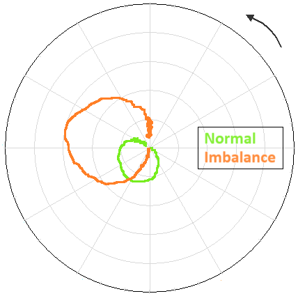
The polar plot shows an increase in amplitude and a phase shift following the event. The phase shift remains constant across all speeds.
Waterfall
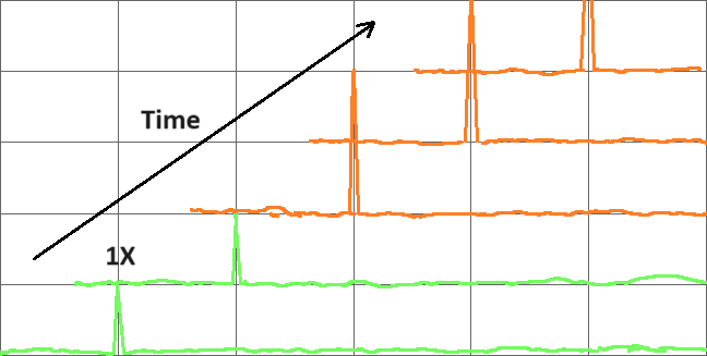
The waterfall plot will show a step change in the 1X amplitude following the event.
Other operational symptoms
The increase in vibration amplitude caused by a sudden unbalance may lead to a rise in bearing metal temperature. If the lost component becomes lodged in the turbine, noise levels may increase, indicated by rattling or broadband noise resulting from flow disturbances.
Machine fault - misalignment
Misalignment generally results in elevated vibration amplitude due to load transfer from one bearing to an adjacent one. This increase typically appears as higher amplitudes at 1X and 2X in spectrum plots, with the 2X amplitude reaching or even exceeding the 1X amplitude as the severity of the misalignment increases. The misalignment may be due to coupling issues or internal misalignment caused by improper bearing elevations.
Amplitude trend
Vibration amplitude trend plots will show increased amplitude in the presence of excessive misalignment.
1X phase trend
1X phase trend will generally be unaffected by misalignment.
Waveform
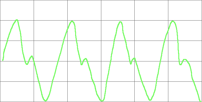
Misalignment will often result in a 2X response. This will be evident in the direct waveform plot as an increase in peak-to-peak amplitude and a prominent 2X frequency component.
Spectrum
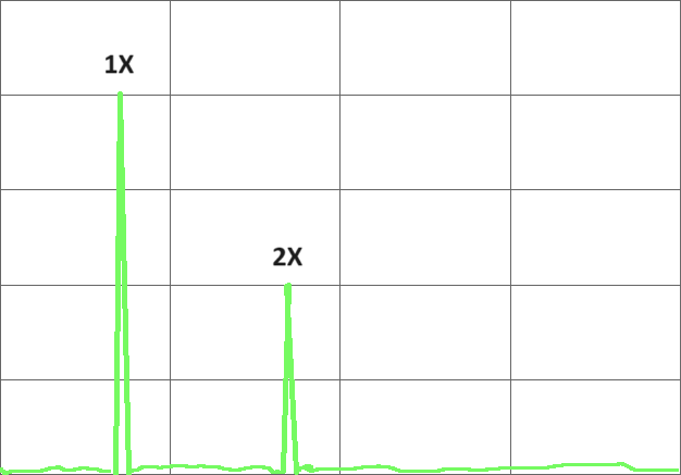
The half-spectrum plot will show elevated 2X vibration in the presence of misalignment. The relative amplitudes of the 1X and 2X peaks indicate the severity of the misalignment.
Full spectrum
The full-spectrum plot will show an increase in the ±1X and ±2X peaks. The positive peaks will generally be higher than the negative peaks.
Direct orbit

The direct orbit plot will show evidence of constrained shaft motion due to misalignment. More severe misalignment may result in an orbit resembling a banana shape, or even a figure-eight.
Shaft centerline

Misalignment may result in a shaft centerline plot that shows the rotor positioned farther from the bearing center. This depends on the severity of the misalignment.
Bode plot - amplitude
An amplitude Bode plot will generally be unaffected by misalignment, aside from an overall increase in amplitude at all speeds compared to a properly aligned machine.
Bode plot - phase
The phase of the Bode plot will remain unaffected by misalignment.
Polar plot
A polar plot will generally be unaffected by misalignment, except for an increase in amplitude at all speeds compared to a properly aligned machine.
Waterfall
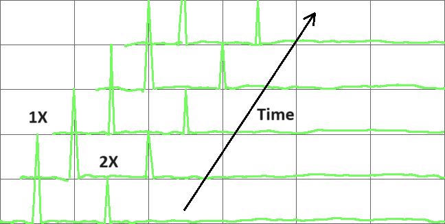
A waterfall plot versus time will show elevated 1X and 2X vibration in the presence of misalignment. The relative amplitudes of the 1X and 2X peaks are indicative of the severity of the misalignment.
Other operational symptoms
Elevated bearing metal temperatures, combined with higher 1X and 2X vibration orders, can be a strong indicator of misalignment. The increased bearing temperature may result from both the higher vibration amplitudes and the additional static load absorbed by the bearing due to misalignment.
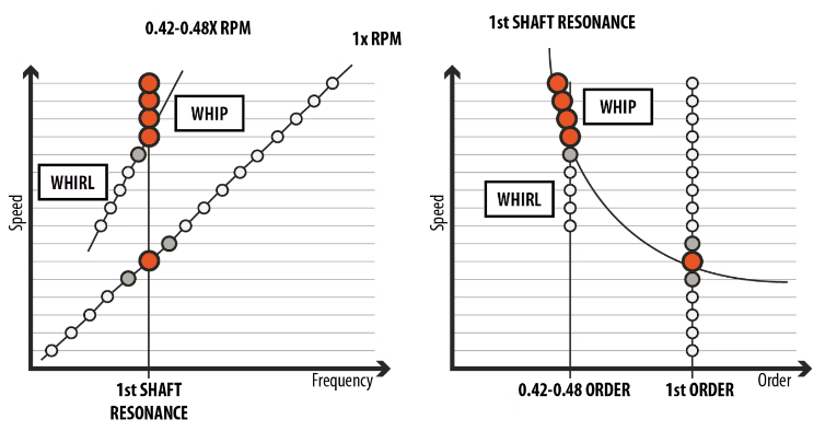
Machine fault - oil whirl
Oil whirl is typically caused by improper design of the rotor-bearing system. The presence of vibration components at frequencies slightly below 1/2X, with varying amplitudes, indicates oil whirl. It can be aggravated by higher speeds, increased oil viscosity, and lighter bearing loads.
Amplitude trend
The overall amplitude trend will typically display a high average amplitude with significant variations in the presence of oil whirl.
1X phase trend
The 1X phase trend will generally remain stable at constant speed in the presence of oil whirl.
Waveform
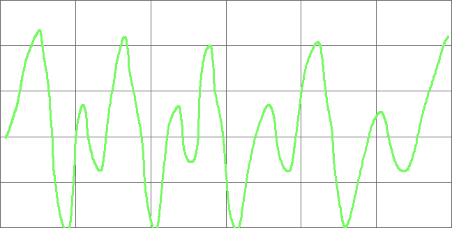
The time waveform plot will show both 1X vibration and a subsynchronous component near 0.48X, with an amplitude that varies over time.
Spectrum
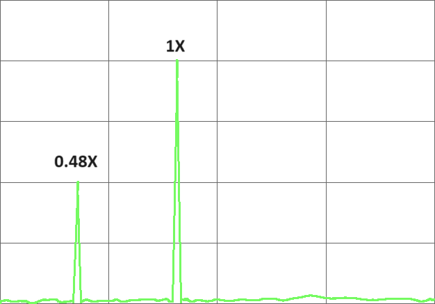
The half-spectrum will show a 1X peak and another peak slightly below 1/2X, which will typically vary in amplitude over time.
Full spectrum
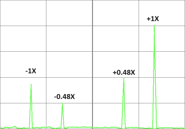
The full-spectrum plot will show forward precession and a subsynchronous peak at slightly below 1/2X.
Direct orbit

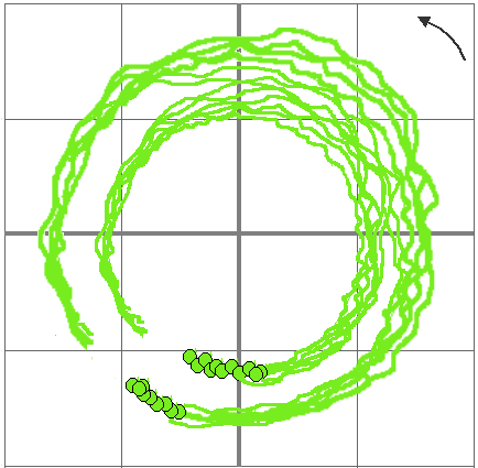
The direct orbit plot will display both the 1X component and a component slightly below 1/2X. The phase marker will gradually shift in the direction opposite to rotation, while the vibration precession will remain forward.
Shaft centerline
The shaft centerline position will generally be unaffected by oil whirl; however, operation near the bearing centerline will be more susceptible to oil whirl.
Bode plot - amplitude
The amplitude plot will generally be unaffected by oil whirl.
Bode plot - phase
The phase will generally be unaffected by oil whirl.
Polar plot
The polar plot will generally be unaffected by oil whirl.
Waterfall

A cascade plot will show the onset of instability, with a subsynchronous peak appearing at a frequency slightly below 1/2X.
Other operational symptoms
Oil whirl vibration may be influenced by changes in the lube oil supply temperature, which in turn alters the rotor dynamic coefficients of the bearing. However, these changes typically have only a limited effect on whirl vibration.
Machine fault - oil whip
Oil whirl will transition to oil whip when the whirl frequency reaches the first natural frequency.
At this point, the subsynchronous vibration locks onto the unstable natural frequency and no longer increases with rotor speed. The vibration amplitude will rise and can become damaging.
Amplitude trend
The overall amplitude trend will exhibit very high values in the presence of oil whip. The amplitude may continue to increase until a limit cycle is reached.
1X phase trend
The 1X phase trend will generally remain stable at constant speed in the presence of oil whip.
Waveform
The time waveform plot will display both 1X vibration and a subsynchronous component at the unstable natural frequency.
Spectrum
The half-spectrum will display elevated 1X vibration and very high subsynchronous activity at the unstable natural frequency.
Full spectrum
The full-spectrum plot will show elevated ±1X components and very high subsynchronous vibration at the unstable natural frequency.
Direct orbit

The amplitude in the direct orbit will increase following the transition from whirl to whip. The precession will remain forward, and the phase marker will shift continuously in the direction opposite to rotation at an accelerated rate.
Shaft centerline
The shaft centerline position will typically be unaffected by oil whip, except that operation near the bearing centerline is more susceptible to oil whirl.
Bode plot - amplitude
A Bode plot (amplitude) will generally be unaffected by oil whip.
Bode plot - phase
A Bode plot (phase) will generally be unaffected by oil whip.
Polar plot
A polar plot will generally be unaffected by oil whip.
Waterfall
A waterfall plot will appear similar to that of oil whirl until the transition to whip. The subsynchronous vibration frequency will then remain constant.
Other operational symptoms
Oil whip can be extremely destructive to the turbine generator. The vibration amplitude will generally increase over time.
Machine fault - operation on resonance
Operating a turbine generator at a critical speed or structural resonance will result in elevated 1X vibration amplitude. This is typically due to a design deficiency but can also be caused by system changes that shift shaft critical speeds, or by structural issues such as foundation degradation, which alter the system’s natural frequencies.
Amplitude trend
The overall and 1X amplitude trend plots will show elevated but stable amplitude at constant speed when running at resonance.
1X phase trend
The 1X phase trend will remain unaffected during operation at resonance and constant speed.
Waveform
The time waveform will display an elevated 1X amplitude.
Spectrum
The half-spectrum plot will display a high amplitude at 1X when operating at resonance.
Full spectrum
The full-spectrum plot will show an elevated +1X amplitude. The −1X amplitude will depend on the ellipticity of the orbit plot.
Direct orbit

The direct orbit plot will display forward precession with elevated amplitude.
Shaft centerline

The shaft centerline position is generally not useful for diagnosing operation at resonance.
Bode plot - amplitude
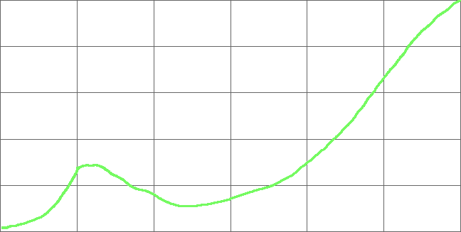
The Bode plot (amplitude) will display elevated amplitude at the operating speed.
Bode plot - phase
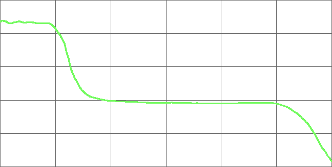
The Bode plot (phase) will display a phase shift as the operating speed is approached.
Polar plot

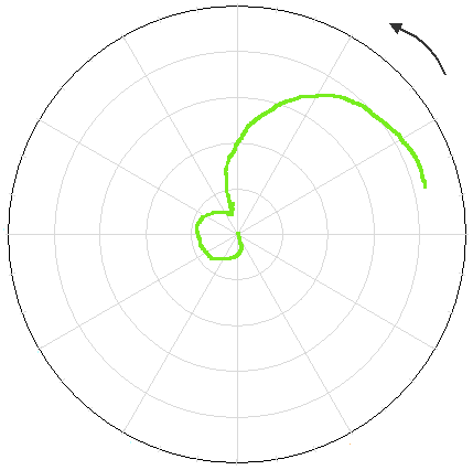
A polar plot will display a phase shift and amplitude peak as the operational speed is approached.
Waterfall

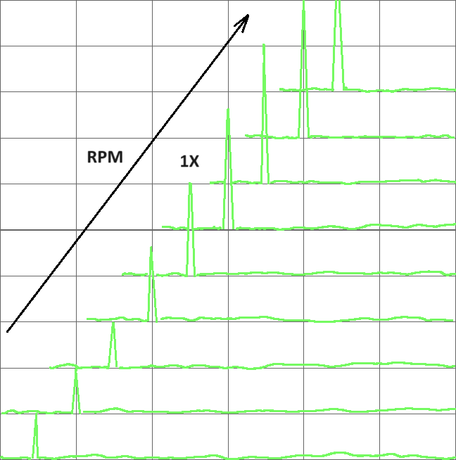
A waterfall plot will display the 1X peak increasing in amplitude as the operating speed is approached.
Other operational symptoms
Measurements from seismic instrumentation can help confirm operation at resonance. If the machine has not previously operated at resonance, changes in foundation stiffness or bearing clearance may cause the structural natural frequencies or rotor-bearing critical speeds to shift into the operating speed range, requiring corrective action.
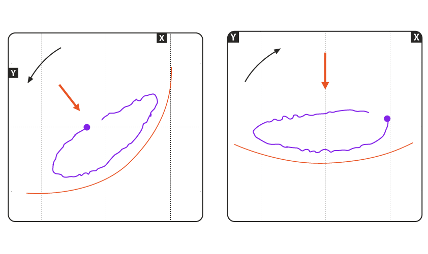
Radial load effect on orbit shape
The orbit plots below represent two different shaft scenarios with opposite directions of rotation.
Both shafts are experiencing high radial loads. The orange arrows indicate the approximate direction of the applied radial load, and the orange arcs represent a section of the bearing wall.
Page 1 of 30