Modal Test & Modal Analysis with DewesoftX

Course overview

This FRF Modal Testing & Modal Analysis course equips engineers and test professionals with hands‑on skills to confidently perform experimental modal analysis using DewesoftX. Starting with fundamental concepts—like FFT‑based Frequency Response Functions and transfer functions—you’ll learn how to excite structures via impact hammer or shaker, set up signal acquisition (triggers, averaging, coherence), and capture high‑quality FRF data.

Next, you’ll define structural geometry within DewesoftX, place excitation and response points, and animate mode shapes to visualize structural dynamics. The course then teaches structured parameter identification: use the modal circle for SDOF systems, and when faced with closely spaced modes or heavy damping, apply multi‑degree‑of‑freedom (MDOF) fitting via the Modal Analysis module to extract natural frequencies, damping ratios, and mode shapes.

Finally, this training walks you through validating and exporting modal models in industry-standard formats (UNV/ UFF) for integration into CAE tools. From acquiring FRF data to building accurate modal models, this course delivers a complete workflow for structural dynamic testing and analysis with DewesoftX.

Frequency response function H(f) in the frequency domain and impulse response function h(t) in the time domain are used to describe input-output (force-response) relationships of any system, where signal a(t) and b(t) represent input and output of the physical system. The system is assumed to be linear and time-invariant. Frequency response function and impulse response function are so-called system descriptors. They are independent of the signals involved.

In the table below you can see typical frequency response function formulations:

The estimation of the frequency response function depends upon the transformation of data from time to the frequency domain. For this computation, we use the Fast Fourier transform (FFT) algorithm which is based on a limited time history. The frequency response functions satisfy the following single and multiple input relationships:

Single input relationship

Xp is a spectrum of the output, Fp is a spectrum of the input, and Hpq is frequency response function.

Multiple input relationship

In the image below we can see an example of two inputs - two outputs case.

Modal test and analysis are used to determine structural modal parameters, such as modal frequencies, damping ratios, and mode shapes. The measured excitation and response (or only response) data are utilized in modal analysis, and then dynamic signal analysis and modal parameter identification are processed. Modal test and analysis techniques have been developed for more than three decades, and a lot of progress has been made. It has been widely applied to the engineering field, such as the dynamic design, manufacture and maintenance, vibration and noise reduction, vibration control, condition monitoring, fault detection, model updating, and model validation.

Modal test and analysis is needed in every modern construction. The measurement of system parameters, called modal parameters, are essential to predict the behavior of a structure.

These modal parameters are also needed for mathematical models. Parameters like resonance frequency, structural damping, and mode shapes are experimentally measured and calculated.

The Dewesoft Modal Test module is what you use when performing structural dynamic test measurements of objects. The Modal Test provides calculated FRF functions (amplitude and phase) over a certain frequency range.

The Dewesoft Modal Analysis module is used after the modal test data acquisition in order to estimate high quality modal models.
The Modal Analysis module uses the results from Modal Test, e.g. FRFs, to estimate modal parameters (resonance frequencies, damping ratios and mode shapes)

The Dewesoft Modal Test module also provides tools to determine modal parameters as well, but these tools only apply for simple structures, having lightly damped and well separated modes. 

Dewesoft Modal Analysis is required to obtain valid modal parameters for complex structures, having multiple resonance frequencies being closely spaced or with heavy damping.

The Dewesoft Modal test module is included in the Dewesoft X DSA package (along with other modules e.g. Order tracking, Torsional vibration, etc.).
The Dewesoft Modal Analysis module comes as a separate license and is not included in the DSA package.   

With the small, handy form factor of Dewesoft data acquisition instruments (DEWE-43, SIRIUSi), it is also a smart portable solution for technical consultants coping with failure detection.

Let's assume there is a mechanical structure to be analyzed. Where are the resonances? Which frequencies can be problematic and should be avoided? How to measure that and what about the quality of the measurement? Probably the easiest way is exciting the structure using a modal hammer (force input) and acceleration sensors for the measurement of the response (acceleration output). At first, the structure is graphically defined in the geometry editor.

Then the points for excitation and response are selected and linked to the defined geometry. The test person knocks on the test points while the software collects the data. Next to extracting phase and amplitude, it is possible to animate the structure for the frequencies of interest. The coherence acts as a measure for the quality. The modal circle display widget provides higher frequency precision and damping factors for modes on simple structures. For additional analysis and for handling complex structures you continue using the modal analysis module. 

If desired the data can be exported to several file formats like the widely used UNV format.

A used example of modal test and modal analysis are shown below:

At first, we have to assume that the methods described here apply to LTI (linear, time-invariant) systems or systems that come close to that. LTI systems, from applied mathematics which appear in a lot of technical areas, have the following characteristics:

• Linearity: the relationship between input and output is a linear map (scaled and summed functions at the input will also exist at the output but with different scaling factors)

• Time-invariant: whether an input is applied to the system now or any time later, it will be identical

Furthermore, the fundamental result in the LTI system theory is that any LTI system can be characterized entirely by a single function called the system's impulse response. The output of the system is a convolution of the input to the system with the system's impulse response.

Transfer functions are widely used in the analysis of systems and the main types are:

• mechanical - excite the structure with a modal hammer or modal shaker and measure the input force excitation together with the output responses from e.g. accelerometer sensors.

• electrical - apply a voltage to the circuit on the input, measure the voltage on the output

For example, in mechanical structures, the transfer characteristics will be able to show dangerous resonances. The frequency range, where the stress of the material is too high, has to be avoided, e.g. by specifying a limited operating range. A simplified process works like this: an input signal x(t) is applied to the system and measured together with the output signal y(t). The division of response to excitation in the frequency domain basically gives the transfer function:

Laplace transformation leads to the result in the frequency domain:

On the picture below we can see a diagram of Laplace transform, which is often interpreted as a transformation from the time-domain (inputs and outputs are functions of time) to the frequency-domain (inputs and outputs are functions of complex angular frequency), in radians per unit time. Given a simple mathematical or functional description of an input or output to a system, the Laplace transform provides an alternative functional description that often simplifies the process of analyzing the behavior of the system, or in synthesizing a new system based on a set of specifications.

How to obtain the transfer function

1. Mechanical structure

2. • Excite the structure with modal hammer or shaker (measure force)

   • Measure the response with accelerometers (acceleration)

3. Electrical circuit

4. • Apply a voltage to the circuit on the input and measure it.

   • Measure the voltage on the output of the circuit

Calculate the transfer function between the measured input and output of the system

Calculate the coherence function. A coherence value of 1 indicates that the measured response is caused totally by the measured input. If the coherence is less than one at any frequency it indicates that the measured response is not only caused be the measured input, but also be additional factors like noise sources.

In order to get started with modal test and analysis, you add the Modal test and (optionally) the Modal analysis modules like indicated in the picture below:

This training material will start with focusing on the Modal Test part, and then we will get back to the Modal Analysis part later on.    

When you add the Modal test module the following setup screen appears:

Test methods

Depending on the application, Dewesoft offers three different Test methods:

Impact Hammer - the structure is excited by impacts from e.g. a modal hammer.

Shaker - the structure is excited by one or multiple modal shakers. The shaker signals can be provided be either Dewesoft AO channels or by other external sources.

ODS - operational deflection shapes, do not use external excitations, but instead the excitations coming from the structure in operation. Hereby, only output response channels are measured. ODS is used for animations of structural deflection shapes, but does not provide a modal model like obtained when using the Impact Hammer or Shaker test methods. 

A modal test method that is relatively easy to configure is when using a modal hammer. The hammer is used for exciting the structure with a short impulse (giving a broadband frequency excitation) and one or multiple acceleration sensors are measuring the response. The hammer has a force sensor integrated and an interchangeable hammer tip that can have different stiffness. Depending of the tip used the frequency bandwidth will be between about 0.5 kHz to 3 kHz. For bigger structures, there are big hammers available with more mass to generate a distinct amplitude. 

The two pictures below show the comparison. The scopes on the top show time-domain, FFTs below show frequency domain (same scaling).

When you have set the calculation type to Impact hammer, the setup looks like the one shown below.

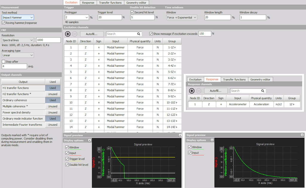
On the Excitation tab, specify the Node IDs where the hammer will hit and on the Response tab the response(s) being acceleration sensor(s) for all Node IDs where they will be located. In the pictures below, we have named the two analog channels Modal Hammer and Acc 1.

FRF channel setup inside Dewesoft data acquisition software

Let's do a short measurement to explain all the parameters. The structure is hit once and the signals are measured.

The hammer signal (upper, blue line) shows a clean shock impact and high damping while the response (lower, red line) starts ringing and smoothly fades out.

Trigger level

The Modal test module needs a start criteria in triggered mode like when using the Impact Hammer method. Therefore we specify a trigger level of e.g. 100 N. Each time the input signal overshoots the trigger level, the FRF calculation (FFT window) will start.

Double hit detection

However, when the input signal shows multiple impulses after one hit (so-called double hits), DewesoftX can identify this if you specify a double hit level. When the signal crosses the double-hit-level shortly after the trigger event, you will get a warning message and can repeat this measurement.

Overload level

You can also enable a warning which will be displayed when the hammer impact has exceeded a certain overload level - when the hit was too strong.

The following picture summarizes the different trigger level options.

Now that we have defined the trigger condition, we should ensure that the FRF calculation covers our whole signal to get a good result.

Window length

Let's assume the sample rate of our example is 10 000 Hz and we have set 8192 lines in the FRF setup.

According to Nyquist, we can only measure up to half of the sample rate (5000 Hz) or the other way round, we need at least 2 samples per frequency line. So, our spectral line resolution is:

The whole FFT window calculation time (block length T) is:

Below you see the cutout data section of the excitation and response signal, which covers pretty much the whole signal.

Note, that the x-axis is not starting at 0 but is scaled in samples from -819 to 15565 due to Pre-trigger settings. In total it gives 16384 samples for each FFT time block,

Pre-trigger

The Pre-trigger time defines how much time prior to the exceeded trigger level that should be included in the FFT blocks. From the screenshot above you can see that 5% of 16 384 samples is 819 samples, which equals t pre = 819 * (1/10 000 Hz) = 81,9 ms. At sample 0 the trigger occurs.

In most of the cases acceleration sensors, microphones, modal hammers or other force transducers are used for analog input. If they are e.g. voltage or ICP/IEPE type, they are connected directly to the ACC amplifier of the SIRIUS data acquisition system, or DEWE-43/MINITAUR DAQ systems with Dewesoft smart sensor interface DSI adapter (DSI-ACC). 

When analog output is needed (for shaker control), the SIRIUS analog out option (8 channels with BNC connector on the rear side of the SIRIUS DAQ system) provides a full-grown arbitrary function generator.

For an easier start, Dewesoft offers auto-generated displays, which already come with the most often used instruments and an arrangement that makes sense for them according to the type of application.

Dewesoft automatically makes 5 auto-generated displays, one for pre-test, 3 for measurements (one for each Test method) and one for analysis.

You should select the visual measurement display that relate to the Test method selected under the MT setup. 

Information and Control section
At the upper left you find display widgets and control buttons that is used to manage the selected Test method. You have clear indication about the time data storing state, information about the measurement state at the current selected sensor groups, option to re-do the measurement at the current sensor groups, select which group of Node IDs that should be measured, and a progress table for the FRF functions to be determined.

Geometry section
At the lower left you find the Geometry widget that will by default show the geometry that was created or imported under the MT setup Geometry tab.

Excitation and response signal section
At the upper right you have the current selected excitation and response channels shown in 2D graph widgets both in time and frequency domain, (time scopes and FFT spectra).

FRF and coherence section
At the lower right you have 2D graphs showing the Frequency Response Functions (FRF) and Coherence Functions (COH).

Depending on the Test method selected the display widgets and controls will be different in order to have the best fit for the configured test. Hereby, there will be differences between all 5 pre-defined visual displays. Also if later on you make chances to the setup, then remember to re-build the visual display in order to update it accordingly to the newest setup changes. You can rebuild the displays by right-clicking on the MT display icon and press Re-build, as shown below: 

Modal test info channels

There are additional channels provided by the FRF module, which give status information during the measurement. To display them, please add a Discrete display in Design mode:

The channels 'Hit status' and 'OVLChannel' can be assigned to it. OVLChannel will only be displayed if the parameter 'Show message if excitation exceed' has been enabled under MT setup first.

FRF control channels

• During roving excitation or roving response measurements, after one group of Node IDs is measured, you can continue to the next group of Node IDs by pressing the Next group buttons.

• If you are unsatisfied with the last measurement, you can cancel it by using Reject last.

• If all measurements in a group must be re-measured, the Reset Group button can delete all the calculated data done for the current group of Node IDs at once.

All the actions are done using control channels in Dewesoft. If you want to create your own visual display then these controls can be modified manually by picking the input control display from the instrument toolbar. Set it to Control Channel and Push-button. Channels Reject last, Next point and Reset point can now be assigned from the channel list on the right.

Force and force + exponential windows

When using triggered test methods like Impact hammer or shaker bursts then you can select between Force and Force + Exponential time windows.
The Window length parameter affects the excitation channels only since the response channels always have a window over the full FFT block length T.
The Window decay parameter is used for the Force + Exponential window type and defines the remaining relative amplitude at the end of the FFT block length.

Force window

A Force Window is a rectangular window with a certain length relative to the FFT block length T.
For Excitation channels the Window length can be adjusted/reduced to only include a part of the duration of FFT block length T, or 100 % of T. In our example the damping is very high (signal fades out quickly), therefore we can select a smaller portion of the signal, e.g. 10 % (usually you would define a noise level first to determine it). Having a window length of 100 % means that all of the acquired data will be taken for calculation (all 16 384 samples of the FFT block in our example from before, the whole block). 

The response signals will always use a Window length of 100 % of the FFT block length T.

Outside the Force window length the excitation signals will be cut out completely, in order to avoid noise.

Force + exponential window

A Force + Exponential window will apply an exponential window on the excitation channels which has a length set by the Window length. After the defined Window length the exponential window drops to zero for the excitation signals.
The response channels will get an exponential window over the full FFT block length, T, no matter the setting for the Window length.
For both the excitation and response channels the Window decay percentage is relative to T.
‘Force + Exponential’ is commonly used for impact testing since it both reduces noise on the excitation and response channels, and keeps equal decay ratios between excitation and response channels inside the defined Window length, which avoids the need for additional window corrections.

The picture below shows how the response window is decayed when different Window decay percentages are selected in Dewesoft .

Averaging of spectra

The result can be improved by averaging the excitation and response spectra over a number of FFT blocks. Therefore, the first e.g. 5 hits in an Hammer Impact test will be recognized and taken into calculation for resulting averaged spectra. After the specified number of spectra are averaged then you move on to the next group of Node IDs.

Roving hammer SISO modal test

In this operation mode, there is one acceleration sensor mounted in a fixed position on the structure. The modal hammer is moving through the excitation DOF points (e.g. doing 5 hits at each point, which are averaged). This is probably the most simple modal test and requires only one hammer and one response sensor. Using a single input excitation and a single output response is referred to as SISO testing - Single Input Single Output testing. 

Roving hammer SIMO modal test

If not all structural modes can be detected by using a single reference DOF (Node ID, Direction and Sign) , then 2 or more response sensors can be used simultaneously at fixed references DOFs, while the modal hammer is roving. This is also referred to as MRIT - Multiple Reference Impact Test.

When using a single input excitation and multiple output responses is referred to as SIMO testing - Single Input Multiple Output testing.

Roving response SISO modal test

The hammer is always exciting the structure in the same DOF position (Node ID, Direction and Sign). Now the acceleration sensor is moved to different DOFs. The disadvantage of this setup is, that the mass of the acceleration sensor changes the structure differently in every point, therefore, influences the measurement (this effect is called mass loading). Also between each measurement, the sensor has to be mounted again, which results in a little more work than when using a roving hammer setup. 

An advantage of using roving response testing is e.g. if it is difficult to impact the structure at all DOFs. 

Using a single input excitation and a single output response is referred to as a SISO test, and if a group of multiple output responses are used (maybe a roving group) then it is referred to as a SIMO test.

Modal shakers are types of vibration shakers used to excite large or complex structures and to achieve high-quality modal data. In comparison to modal hammers, modal shakers have the ability to excite the structure in a broader frequency range, and with many different signal types, best suited for different structures and ideal for accurate test results. Shaker tests are often used for critical structures and when extended analysis is required. Shaker testing often use a large group of response sensors.

The channel setup of a SIMO shaker modal test is shown below:

MIMO shaker setup

The channel setup of a MIMO shaker modal test is shown below:

If the shaker is externally controlled, Dewesoft offers Burst mode (triggered acquisition) or Continuous mode (free-run acquisition):

Continuous shaker excitation type

In Continuous mode spectra are calculated continuously as data are acquired throughout the measurement. A list of time weighting FFT windows for continuous signals are supported, and the calculated spectra can be set to overlap in time by specifying the Signal overlap parameter. 

The calculation runs to the end of the measurement, but it can also be stopped automatically after a user-defined number of spectra by Checking on the ‘Stop after’ parameter under FRF settings, and specifying a number of averages. 

Burst shaker excitation type

In Burst mode the calculation of each spectrum is triggered by the externally controlled excitation signal. When the excitation input signal exceeds the Trigger level a new spectrum will be calculated. Depending on the ramp-up burst time, a Pre-trigger can be adjusted to ensure the FFT block of time samples, used for a spectrum, includes the entire burst. 

Time window functions for burst random signals are supported together with related user-defined window parameters. With triggered spectrum calculation Signal overlap is disabled since it is controlled by the trigger.

If the shaker is controlled with Dewesoft AO, we support Continuous random, Burst random and Sine sweep generator output excitation signals. AO is an abbreviation for Analog Output. All the settings for the function generator can be done directly in the Modal test setup. 

For all Waveform types the AO soft start and soft stop times can be set. The soft start/stop times define the duration of half-sine leading and trailing gain tapers. The measurements will be calculated after the leading taper and before the trailing taper, except for triggered calculations when using Burst random. 

In the Excitation channels table the Dewesoft AO channels to use must be selected, and their output voltage target amplitudes must be set. The Dewesoft output channels will have the defined voltage target amplitude over all frequencies. 

Continuous random waveform

By selecting the Waveform type Continuous random, AO channels will output continuous random noise. The random noise will have a frequency Bandwidth equal to the Nyquist frequency of the DAQ device's sample rate, where the Nyquist frequency is given by:

Burst random waveform

With Burst random Waveform type, the AO channels will output bursts of random signals with a user-defined burst length. The burst length (between the AO soft start and stop times) is set by the Excitation duration parameter. The excitation duration is specified in percent of the FFT time block length used for each spectrum:

Note: For minimum spectral leakage, remember to limit the Excitation duration enough to have room for the AO soft start/stop times in the FFT time blocks. Also, make sure the Pre-trigger is set such that the FFT time block includes the entire burst - from the beginning of AO soft start to the end of the AO soft stop:

Sine sweep waveform

The Sine sweep waveform outputs a sinusoidal signal that sweeps in frequency from Start freq. to Stop freq. over a specified Sweep time or with a specified Sweep rate. The frequency sweeping will begin after the AO soft start time and end before the AO soft stop time.

Swept sine testing will typically provide great coherence between input and output, and the total input force to the structure can be kept relatively low since only one frequency is excited at the time. 

When using Sine sweep with multiple shakers, multiple sinusoidal sweeps have to be measured to be able to un-correlate the multiple input excitation signals. To be able to distinguish between the multiple excitation signals, the excitation pattern has to be different between the sweep runs.
In Dewesoft, this is managed by changing the phase pattern between sweep runs for the AO channels. Each sweep will have a phase profile containing the phase for each AO channel. The profiles can be set randomly by pressing the button Randomize profiles, or it can be set by the user in the Excitation channels table. 

In order to un-correlate the excitation signals, at least the same number of sweep runs as the number of included AO channels must be used. The multiple phase profiles should be as different as possible to get best results.
For example using two AO channels the optimal phase profiles are 0° and 0° for run 1, and 0° and 180° for run 2.

The measurements are averaged over all sweep runs, hereby measured data from all phase profiles are used for the spectral results.

No phase profiles need to be configured for the random waveform types, since the excitation patterns between AO channels already change by the independent noise signals

You should ensure that the sweep is slow enough because the FFT needs some time T for calculation (dependent on the number of lines, resolution). . The settings for the Dewesoft AO signals are the same as under the Function Generator module.

When you switch to Measure mode or press the Store button, the sweep will start.

When using a sine sweep, as the sweep moves through the frequencies, the graph data will be updated. Putting the AO/Freq channel on a separate display is a good way to show the current frequency.

The picture above shows two 2D graph instruments with transfer functions 2-1 and 3-1 (amplitude on top and the phase below) during a sweep. The left side is already calculated while the right side is ongoing.

Operating Deflection Shapes (ODS) is a simple way to do dynamic analysis and see how a machine or a structure moves within its operational conditions. ODS tests have no applied artificial forces and only response vibration signals are measured. 

Dewesoft supports two ODS types:

• Time ODS - used by adding a separate Time ODS module to your DewesoftX setup.  

• Frequency ODS - included in the Modal Test module as one of the Test methods.

Time ODS calculates deflection shapes over time, over a time axis, opposite to Frequency ODS which calculates deflection shapes over a frequency axis.
In this way, you can see how the overall structure deflects at a specific time instance with Time ODS, and you can see how the structure deflect at a specific frequency by using Frequency ODS.

Time ODS

The time ODS module can be added to the setup file like shown in the picture below:

In the Time ODS setup you can select vibration channels as inputs, being acceleration, velocity or displacement channels, and you can Integrate or differentiate them to obtain e.g. displacement as the output quantity. A geometry can be created in the same way as in the MT module. 

For more information about Time ODS please use the following links:

• Time ODS Online Help

• Modal Test and Analysis Manual - Time ODS section

Frequency ODS

When performing Frequency ODS, one of the accelerometers has to be set at a reference channel in order to calculate phase information. In Dewesoft this is done by selecting the reference response sensor as an excitation channel. The reference channel should be placed at the DOF revealing the most structural modes. 

In you want to group your sensors and move them during the measurement, select option Roving response.

This will create different groups and you can manually select the sensors in the same group or change group names.

During the measurement, you can switch between the groups:

In the experimental modal analysis (EMA), the structures are excited by artificial forces and both the inputs (excitation) and outputs (response) are measured to get the frequency response functions (FRF) or impulse response functions (IRF) by digital signal processing. Modal parameters can be identified from FRF or IRF by identification algorithms in the frequency domain or the time domain. EMA tests are usually carried out in the lab, with the advantage of high signal to noise ration (SNR) and easy to change test status.

EMA identification methods can be classified into a time domain (TD) methods and frequency domain (FD) methods according to different identification domain. Also, they can be classified according to a different number of input and output:

• SISO (single input single output),

• SIMO (single input multiple outputs),

• MIMO (multiple inputs multiple outputs).

The FRF is generally utilized for the EMA in the frequency domain, which is estimated from the excitation and response signals. Then the modal parameters are identified by constructing the parametric or nonparametric models of the FRF and curve fitting them. The IRF is generally utilized for the EMA in the time domain. It can be obtained from the inverse FFT of FRF.

Time domain methods are suitable for the global analysis in a broad frequency band, which have good numeric stability. However, there are some limitations too:

• very difficult to confirm the order of math model,

• always time-consuming,

• many calculation modes got with the structural modes and difficult to delete them,

• many settings needed, complicated-to-use,

• not being able to take into account the influence of out-band modes.

On the opposite side, frequency domain methods are always reliable, rapid, easy-to-use, with the capacity to consider the out-band modes and analysis uneven spaced FRFs, so they are applied widely.

Operational modal analysis is used for large civil engineering structures, operating machinery or other structures, making use of their output response only. These structures are always loaded by natural loads that cannot easily be controlled and measured, for instance, load from waves (offshore structures), the wind loads (buildings) or traffic loads (bridges).

Both OMA and ODS only use output response channels, but where ODS mainly provide deflection shapes for animation, OMA provides a modal model like EMA (Experimental Modal Analysis) does, which includes resonance frequencies, damping ratios and mode shapes of simple and complex structures.

When it is possible EMA is typically preferred over OMA as the best modal test type due to the controlled environment, where the operator can manage the structural excitations. But, in cases where it is difficult to excite the structure by artificial means, OMA is a great way to go. Moreover, all the measured responses come under operational state of structures, and their real dynamic characteristics in operation could be revealed, so OMA is very suitable for health monitoring and damage detection of large-scale structures.

Multiple-Input Multiple-Output (MIMO) measurement techniques are a well-proven and well-established method for collecting FRF data sets. MIMO methods offer some distinct advantages for the measurement and extraction of basic modal parameters especially while testing larger structures. 

The main advantage of MIMO is that the input-force energy is distributed over more locations on the structure. This provides a more uniform vibration response over the structure, especially in cases of large and complex structures and structures with heavy damping. In order to get sufficient vibration energy into these types of structures, there is a tendency to overdrive the excitation DOF when only a single shaker is used. This can result in non-linear behavior and deteriorates the estimation of the FRFs. Excitation in more locations often also provides a better representation of the excitation forces that the structure experiences during real-life operation.

The response transducers must be roved around unless there are sufficient transducers available to cover all the response DOFs. With this type of testing, uncorrelated random (continuous, burst, or periodic random) excitation signals are used. Burst random and periodic random signals have the ability to provide leakage-free estimates of the FRFs, i.e., without resolution-bias errors, which is an advantage compared to continuous random signals.

A demo measurement was done on a plane model. The structure was excited by two shakers with uncorrelated excitation signals. The responses were measured with 3-axial accelerometers and the excitation signals were measured with force transducers. The voltage signal for the shakers was supplied from the Dewesoft Function generator (AO module).

On the left side of the Modal test UI, you select Shaker as a test method, resolution of the measurement, and additional output channels.

On the right side of the UI, define the excitation source and excitation channels. We will use Dewesoft AO to drive the shakers and we select Burst random noise as the type of excitation. 

We will measure the excitation with 2 force transducers in Z+ direction, at points 1 and 2.

We measured the responses with 4 tri-axial accelerometers in X, Y, and Z direction (points 1, 2, 4, 5) and with 2 uni-axial accelerometers in Z direction (points 3 and 6). Setup was done accordingly, as shown in the image below.

On time-domain recorder (top right corner) you can see time domain channels from excitation and responses.

On the left side, the results are displayed on 2D graphs. You can see transfer functions, coherences, and MIF (mode indicator functions). The geometry is animated from the selected frequency.

The transfer functions tab gives an overview of which transfer functions that will be calculated. For large test setups involving many sensor locations and multiple references the full set of transfer functions can be big. If not all transfer functions are required while performing measurements they can be toggled from ‘Used’ to ‘Unused’ to increase the performance. In Analyze mode, when doing post-analysis, the ‘Unused’ transfer functions can be toggled back to ‘Used’ and recalculations can be done based on the acquired time data. 

Under the Geometry editor tab you can create or import a geometry that relates to the test. The geometry is mapped to the channels via the Node IDs. After connecting all nodes to channels the geometry can animate mode shapes and defection shapes depending on the used Test method.
For additional information about how to use the Geometry editor please look at:

• Geometry online help page

• Modal test and analysis manual

The geometry can be managed in the Modal Test setup under the Geometry editor tab, or in Measure we can add the “Modal Geometry” widget.

When the Geometry editor tab is used under the Modal Test setup, the geometry are automatically shown on the pre-defined measure displays for MT.

Importing geometries

You can Import UNV / UFF (universal file format) geometries from other software (e.g. MEScope or Femap) into DewesoftX. Of course, you can also import a geometry that was drawn in DewesoftX's FRF Editor before. You can also use Load to open geometries from XML files. 

On the Geometry tab on the Modal test setup, or from the properties of the Modal geometry widget on the left, select Load of Import.

Drawing a structure

To draw a structure go to the Geometry editor tab in the Modal Test setup. In the editor we can add Objects, Nodes, Lines and Surfaces. All the points and objects can individually be defined in a Cartesian coordinate system or Cylindrical coordinate system.

Objects

The structure can be assembled from pre-defined objects. The object that are available in the Geometry editor are:

• Cuboid

• Plate

• Circle

• Sphere

• Cylinder

• Cone

For each object you can define the position (X, Y and Z coordinate), size (of axis) and number of points in each axis. If the user selects option Surfaces, the surfaces will automatically be assigned to the structure.

Nodes

Under the Nodes tab in the Geometry editor you can link the channels, used in the setup, to the geometry. The setup channel Node ID numbers are linked to the geometry Node ID numbers. Nodes are points where the sensor is positioned on an object.

Nodes are defined with location (X, Y, Z) and rotation around axes (X angle, Y angle, Z angle). In order to create a new structure from nodes, we have to switch to the Nodes tab. Now we have to create a coordinate system in which we will define our nodes. This can either be Cartesian or Cylindrical. After the coordinate system is created, we can add nodes with the Plus button.

After nodes are created we can change their rotation (according to how the sensor is rotated on the object) with all three axes. Nodes can be selected with selection in the node table or with the right mouse click on the structure preview window. When a node is selected, rotation is shown with a small coordinate system located directly on the node. In the picture below you can see a selected and rotated node. 

Lines

When nodes are defined we can go ahead and manually add lines to connect them. An easy way to create lines is to right click with the mouse on the node, select Add -> Lines.

Left click on the first node and move to the second node. This will create a white line and when you hover to the node, the line will change to green color. Select the second node and the line will be added. You can add multiple lines consecutively. Right mouse click will stop adding lines. 

If we don’t want to draw a connected line, we can also manually add lines by pressing on the Plus button in Lines tab of the Geometry editor.

Surfaces

Surface can be defined with 3 nodes. Triangle surfaces can be added with a right mouse click on a node point, Add -> Triangles.

Triangle surfaces can also be added by clicking the plus button and manually defining corners. 

Cartesian coordinates

Cartesian coordinates Usually nodes are presented with a Cartesian coordinate system. This means you have X, Y, Z position and rotation around all three axes. Coordinate system can be used for grouping nodes, because you can later rotate or translate them with the Center point. 

Cylindrical coordinates

Cylindrical coordinate system is used for easier creation of round objects. Points are defined with radius, angle and z (height) around coordinate systems center point. Cartesian and cylindrical CS can be combined in one geometry.

When it comes to importing a more complex geometry into the DewesoftX's FRF geometry editor, the number of nodes can be very large. If you are using a CAD software solution that do not support export to UNV and do not support reduction in the number of node points, then you can find a freeware-converter GMSH from e.g. STL-to-UNV here: http://geuz.org/gmsh/.

After downloading it, open the program. Then you can open any STL file.

The geometry will be seen in GMSH.

The click on Save as and choose *.unv file format and rename the file to .unv.

After that, import the geometry in DewesoftX in the same way as it is described on the previous page.

All the nodes and triangles are defined in the .unv file format.

Geometry is now ready to be used for modal animation.

For the following explanation of parameters, a triggered FRF was done on a snowboard structure. All 39 excitation points were sequentially hit by a modal hammer and relate to one reference response accelerometer.

Only 1 hammer and 1 sensor were used.

From the channel list on the right side, we see that each point (#1, #2, #3, #4) is related to the reference point (#1). For each excitation point, a transfer function was calculated, e.g. TF_1Z+/3Z+. 

FRF functions consist of amplitude and phase information, or real and imaginary information, over a defined frequency range. The 2D graph is the graph widget to use for illustration. you can select what you want to display by using the properties from the left side.

To make a bode plot, use two 2D graphs below each other. The above one shows the amplitude (y-axis type: LOG), the lower one the phase (y-axis type: LIN).

When the amplitude of the transfer function shows a local maximum, and the phase has turned around 90 degrees at this point, it usually indicates a resonance. But to avoid an erroneous statement, other parameters have to be checked as well.

The coherence is used to check the correlation between output spectrum and input spectrum. Thereby, you can get indications of the power transfer between input and output of a linear system. Easily talking, it shows how good the input and output are related to each other. 

The amplitude of the coherence goes from 0 to 1. Low values indicate a weak relation between input and output channels (e.g. due to noise or when the excitation spectrum has gaps at certain frequencies), and values close to 1 indicate good representative measurements.

NOTE: Coherence results must be based on averaged measurements. In the case no averaging is used the coherence will always show an incorrect value equal to 1.

If the transfer function shows a peak, but the coherence is low (orange circles in the picture below), it might not necessarily be a real resonance. Maybe the measurement has to be repeated (e.g. with a different hammer tip?), or you can additionally look for the MIF parameter, explained below.

Coherence is calculated over the frequency range and can be illustrated in a 2D graph widget.
Coherence channels are calculated separately for each point (e.g. Coherence_3Z/1Z, Coherence_4Z/1Z, …).  

The coherence function indicates the degree of a linear relationship between two signals as a function of frequency. It is defined by two autospectra (GAA, GBB) and a cross-spectrum (GAB) as:

For more information about autospectra and cross-spectra please look up:

• FFT Analysis Pro-training, Auto- and Cross-spectra

• FFT Analysis Ultimate guide, FFT Results

At each frequency, coherence can be taken as a correlation coefficient (squared) which expresses the degree of the linear relationship between two variables, where the magnitudes of autospectra correspond to variances of those two variables and the magnitude of cross-spectrum corresponds to covariance.

There are four possible relationships between input A and output B:

• Perfectly linear relationship

• A sufficiently linear relationship with a slight scatters caused by noise

• Non-linear relationship

• No relationship

If all parts of a structure are moving sinusoidally with the same frequency (fixed phase relations), this motion is called normal mode. This happens at resonance or natural frequencies. Depending on the structure, material, and bounding conditions there exist a number of mode shapes (e.g. twisting, bending, half-period, full-period movement...).

These are usually calculated using finite element simulation software, or/and by experimental modal measurement and analysis.

As mentioned earlier, when the amplitude of the transfer function shows a local maximum, and the phase is turning at this point, it usually indicates a resonance. To be sure, also the Coherence should be checked as described before. And last, you can look at the MIF (Mode Indicator Function).

In Dewesoft a MIF value close to 1 indicates a mode shape.

The spikes shown in the picture below are very likely resonance frequencies. Just click on them and check the movement in the geometry instrument.

The MIF function has values at all spectral lines should be displayed with a 2D graph widget.

The MIF is calculated from all FRF functions (all DOFs are included), and therefore the result is only one channel.

Note: in other SW applications the MIF is often shown by having valleys at resonances instead of peaks. In Dewesoft we use 1 - MIF compared to such other SW, in order to get modes indicated with peaks.

The structure movement animation is done by putting sine functions with the amplitudes and phases from the measurement into the geometry model points. The animation is done in one direction (in our example Z+). For FRF and Frequency ODS results you can animate the structure for a single frequency, which can be chosen in the 2D graph when setting the Cursor type to Channel cursor, as shown below.

Note that for Time ODS it is the time cursor in the Recorder widgets that will determine the time instance for the shown deflection shape.  

Other than that, the frequency can also be chosen manually in the modal geometry widget properties on the left.

Different parameters like animation speed and amplitude (scale), as well as the visibility (nodes, point numbers, traces, shapes, coordinate system axes), can be changed here.

Here are some of the mode shapes of the snowboard calculated by DewesoftX Modal Test, where you can see bending and twisting/torsional modes.

Finally, when you are certain that the point you are looking at is a resonance, you might want to get its exact frequency and damping factor.

As the FFT can never be that precise (high line resolution needs long calculation time, which is not given when there is a hammer impact), there are some mathematical methods to interpolate.

In the Dewesoft Modal Test module, the circle-fit principle method is included. The modal circle method can be used for simple SDOF structures having few, well separated, and lightly damped modes. 

If more complex structures has to be investigated the Dewesoft Modal Analysis module should be used. The Dewesoft Modal Analysis module includes more advanced modal parameter estimation techniques capable of analyzing complex MDOF structures having many, closely couple, and heavily damped modes.
The Modal Analysis module features will be described later in this Pro-training material.

Circle fit analysis procedure

The FFT lines to the right and left side of a peak (so-called neighbor lines) are drawn by real and imaginary parts in the complex coordinate system. A circle is aligned between them with minimum error to each point and the resonance frequency is approximated.

The geometrical interpretation of the formula for the mobility FRF of damped SDOF system is a plot of Im(Y) vs. Re(Y). The picture below shows the mobility FRF of the damped SDOF system (Amplitude) and the Modal circle plot on the right side.

The selected point in the FRF curve should not be influenced by neighboring modes. The circle arc should be around 270 degrees.

The damping ratio is calculated using a user-defined number of points in the circle below and above resonance.

Imagine that we had a sample rate of 2000 Hz, and 1024 FFT lines, resulting in a line resolution of 0.977 Hz. The peak, that we are looking at, is at 73,2 Hz. But it could be in the range of 73,2 Hz ± 0,977 / 2 Hz. In the example below, we switched the 2D graph's Graph Type property to histogram to make the FFT lines visible.

We add the Modal circle from the widget toolbar. The 2D graph is again in cursor mode, the modal circle widget will follow. By clicking on the peak, at first, no resonance peak is found.

Then we increase the Peak search range from 10 Hz to 20 Hz. The peak is found and by changing the neighbor count you can select how many FFT lines left and right from the peak are taken into calculation. The points should all be aligned nicely on a circle. The small red circle point shows the calculation result in the Modal circle widget.

Our final result shows 72,775 Hz and a damping factor of 0,038. With these parameters, one can proceed further in the Dewesoft Modal Analysis module or in other simulation software.

As mentioned in the beginning of this training material, the Dewesoft Modal Test module is what you use when acquiring structural dynamic test data of objects, which provide calculated FRF and other modal related function types.

The Dewesoft Modal Analysis module is used in Analyze mode, after the modal test data acquisition, in order to estimate high quality modal models.
Where Dewesoft Modal Test mainly provide tools to determine modal parameters of simple structures, having lightly damped and well separated modes, Dewesoft Modal Analysis provide tools to determine valid modal parameters for complex structures, having multiple resonance frequencies being closely spaced and with heavy damping.

The Dewesoft Modal test module is included in the Dewesoft X DSA package (along with other modules e.g. Order tracking, Torsional vibration, etc.).
The Dewesoft Modal Analysis module comes as a separate license and is not included in the DSA package. 

Why estimate a modal model?

Why use the Modal Analysis module to estimate modal parameters instead of just using the parameter values found with the tools from the Modal Test module? This depends on the test structure, if it's structural dynamic behaviors are relatively "simple" or more "complex".

SDOF (Single Degree Of Freedom) Fitting
SDOF curve fitting (supported in the Modal Test module) can be used on simple structures with well-separated modes having only small mode overlaps, or at certain frequency bands where the structure fulfills such requirements. At resonance frequencies simple structures will behave like a SDOF system. For SDOF systems the Modal Circle widget can be used to indicate acceptable resonance and damping values.

When structures are lightly damped (<1 % damping) this often causes the present modes to have small overlaps - the modes are said to be lightly coupled. 

MDOF (Multi Degree Of Freedom) Fitting
MDOF curve fitting (supported in the Modal Analysis module) should be used on complex structures with closely spaced modes and with heavily damped modes which cause overlaps between modes. MDOF curve fitting can be used at certain frequency ranges where such characteristics occur or over the full frequency range.

MDOF fitting is done by estimating a modal model, which can separate all modes (also overlapping modes) from each other and hereby determine valid modal parameters even though the modes are closely couple. This is not possible for the SDOF fitting methods.  

Modal parameter estimation becomes relevant when measured FRFs contain overlapping modes. If modal parameters for complex structures are estimated as being SDOF systems (by using e.g. the Modal Circle fit method and quadrature picking), then other modes close by will affect the mode estimation and results will be inaccurate.

In order to estimate modes of complex structures without getting affected by other closely coupled modes, MDOF curve fitting is used where a series of SDOF systems are optimized to fit/mimic the CMIF best possible. The number of SDOF systems in the final estimated model is based on the number of poles (and hereby modes) selected on the Stabilization diagram.  

By being able to describe measured FRFs (that have a mix of overlapping modes) with a series of SDOF systems, it becomes possible to accurately estimate each mode without they are being affected by other nearby modes.

One of the main parameters used in curve fitting is the Order, also referred to as Iterations or Modal Size, which defines the polynomial order of the fitted mathematical function. Order needs to be set high enough to be able to fit the function to all modes included in the selected frequency range/band, and also high enough to compensate for the residual effects of modes that lie outside of the selected curve fitting band.
But if the fitting order is set too high, the fitting function will begin to fit noise in addition to the modes and will represent non-physical Computational Modes as well.

In order to get started with DewesoftX Modal Analysis, add the Modal analysis module like shown below:

Note that modal analysis output channels will only be calculated after measurements has been acquired, using the related datafiles in Analyze mode. 

The modal analysis setup has a table containing added FRF functions to the left and General settings on the right side. 

Transfer functions table

In the Transfer functions table you must add the measured FRFs you want to use from Modal Test. This can be done either by pressing Add all TFs, which will import all measured FRFs in the datafile, or by pressing Add, which will add one row to the table for you to assign an FRF to. 

The measured FRFs you want to include in the modal model estimation process should be set to Used -> True.

The Transfer function preview tab will show the FRFs that are set to Preview - > Enabled (>>) which can help with determining the relevant frequency range to include for the estimation proces. The Preview will also illustrate which modes are present between all FRFs (global modes) and which are only found at one or few FRFs (local modes).

When performing global mode curve fitting all FRFs should contain the global modes. Otherwise, the global estimation might be inaccurate.

General settings

Under General settings you start with selecting the frequency range for the analysis. Maybe the full range must be analyzed or maybe only a certain frequency region is of interest.

The Damping correction parameter should be enabled if you have used the Force + Exponential FFT window for the measured FRFs.

Calculations tab

Under the Calculation tab you can adjust settings for the Stabilization Diagram, and which output functions you want to include. We will get back to the Stabilization diagram in the next section.

• Max order - Increasing the order of the curve fit will also increase the number of calculated poles to select between in the Stabilization diagram. When the calculated poles begin to only change a little between individual neighbor orders, then the poles are said to be stable.

• Frequency tolerance - Defines the limit for how much neighboring poles must deviate in frequency in order to be Frequency stable poles.

• Damping tolerance - Defines the limit for how much neighboring poles must deviate in damping to be stable poles with respect to damping. 

The Outputs section determines which output functions that will be calculated. Offline means that the function is calculated in Analyze mode - like we do when using the Modal Analysis module. The function type will not be calculated if it is set to Unused.

• CMIF - Complex Mode Indicator Functions (CMIF), have one function for each reference DOF included (poly reference) and can help identifying closely coupled modes and repeated roots. CMIF is based on Singular Value Decomposition (SVD) of all the Used FRF functions, to identify all modes included in the model test measurements. The CMIF functions have peaks at resonances - indicating poles of the DUT.

• FRF synthesis - FRF Synthesis is used as a validation tool by comparing the FRFs from the estimated modal model (the synthesized FRFs) with the real measured FRF data.

• Mode shapes - Outputs the mode shapes for the modes selected on the stabilization diagram - based on the estimated modal parameters.

• AutoMAC - The Modal Assurance Criterion (MAC) is used to determine the similarity of two mode shapes. "Auto" in AutoMAC means that the two mode shapes comes from the same test.

You use the Stabilization Diagram (or SD) to determine what the modal parameter identification should be based on. It helps with identifying stable poles and thereby consistent modes which can be used for the modal parameter estimation process.

The poles consist of the modal frequency and damping. When the poles are green circles it fulfills the tolerance settings for stable frequency and damping, as specified under General settings in the Modal Analysis setup. 

You must select a stable pole from each mode you want to estimate, by left-mouse-clicking on the poles. When the set of poles are selected press the Recalculate button and estimation process will be done, as shown below: 

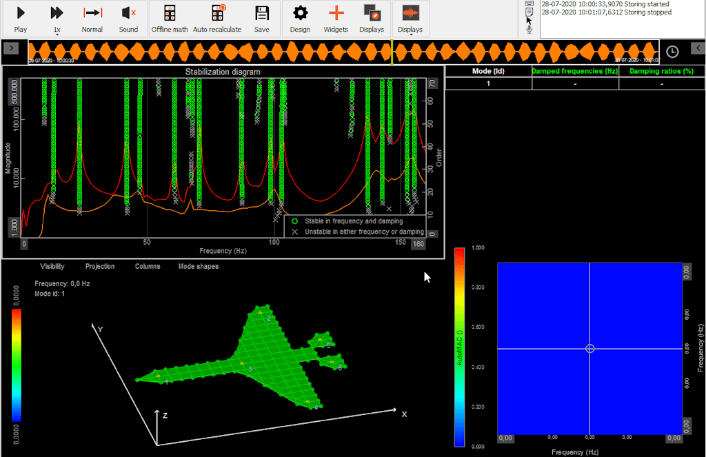
On the stabilization diagram you can also display the CMIF curve(s) which help with overviewing the detected structural modes when you are selecting poles for the estimation process. CMIF is based on Singular Value Decomposition (SVD) of all the Used FRF functions to identify all modes included in the model test measurements. The CMIF functions have peaks at resonances - indicating poles of the DUT.
CMIF outputs one function for each reference DOF included.

The stabilization diagram can be added to the Analyze - Review display by adding the widget as shown below:

When stable poles have been selected on the stabilization diagram and modal parameters have been calculated, you should validate that the quality of the results by using Modal Assurance Criteria (MAC) and by comparing the synthesized FRFs with the measured FRFs. If both MAC results and the synthesized FRFs looks good, then you have obtained representative resonance frequencies, damping ratios and mode shapes for the individual modes of the structure - even though some modes are closely coupled.

AutoMAC

AutoMAC is used to verify that the selected and estimated modes can be distinguishable with the amount of FRFs used. If too few DOFs are measured two different modes might behave in the same way at the DOF nodes being measured. In such cases multiple modes are not distinguishable and the modal estimation might mix mode information together. 

To ensure an acceptable spatial resolution, enough DOFs must be used to detect unique mode characteristics for all modes. Also, the DOF node positions have to be chosen in ways that detects all those modes and their differences between each other.

The AutoMAC results has a value between 0 and 1 for all mode pairs. A value of 1 means that the pair of modes are 100 % correlated, and a value of 0 means that the mode pair do not have anything in common. In the picture below you see an AutoMAC of a modal model with 9 modes. The diagonal mode pairs (mode 1:1  ,  2:2  ,  ...  9:9) will always have a value of 1 since the modes will always be 100 % correlated with itself. On the other hand, off-diagonal values (e.g. mode 1:2 and 3:5) should be as low as possible to indicate that the estimated modal is based on data with distinguishable modes.  

Synthesized FRFs

FRF synthesis is a validation tool used by comparing the FRFs from the estimated modal model (the synthesized FRFs) with the real measured FRF data. It is therefore possible to see how well the estimated model mimics the dynamics of the physical structure. If the synthesized FRFs looks similar to the measured FRFs it verifies that the modes of the measured structure can be described by the estimated model - This means that it has been possible to describe the structure successfully with a series of SDOF systems, which have well defined modal parameters.

Mode shapes

The mode shapes are estimated by an LSFD (Least-Squares Frequency Domain) method. The LSFD performs local estimates based on individual FRF measurements together with the Global modal parameters (frequency and damping), which were estimated by the MDOF global curve fitter.

The mode shapes for each mode are vectors consisting of complex values for each DOF point. The complex values describe how the DOFs are moving relative to each other for a certain mode. In the illustration below estimated mode shapes of a complex structure is animated. For each estimated mode a mode shape vector is determined and used for animation.    

Mode shape animation can help you with verifying the how the estimated modal describe the measured FRF data and FEM models by comparing the animations of measured or analytical FRFs with the estimated mode shapes.

After the measurement is done the data can be exported to a lot of different file formats, e.g. UNV/UFF, Diadem, Matlab, Excel, Text... The modal data results can be separately exported by Real, Imag, Ampl or Phase parts, whatever you prefer.

In MS Excel, for example, FRF data will appear on a sheet called Single value. For each FRF, Real/Imag/Ampl/Phase is exported.

If you prefer it differently, data rows and columns can simply be exchanged in MS Excel by copying and using the Transpose function from the submenu when pasting.

The Universal File Format (also known as UFF or UNV format) is very common in modal analysis. Depending on the header, it can contain either transfer functions, coherence, geometry, ... or various other data.

The following example shows how to export data recorded by Dewesoft into Vibrant Technologies ME Scope analysis software and how to display it there.

First, choose the UNV export from the export section and the option Export complex channels if you want to export phase, real and imaginary part. Then select all your transfer functions (you can use the Filter and type TF for simplification). When clicking on the Export button you will create a UNV datafile.

In the Geometry editor the structure can also be exported separately to the UNV format. This creates the UNV geometry file.

UNV files can be imported to a software application supporting UNV files (like ME Scope, N-Modal, ...). In ME Scope click File -> Import -> Data block. Then select the UNV datafile.

The transfer functions are now illustrated.

Then click File -> Import ->  Structure and select the UNV geometry file.

Now both data and geometry are successfully imported into ME Scope. Let's try to animate it, select Draw -> Animate Shapes.

A pop up appears, and we select to match the structure and transfer data. Equations are created.

Finally, you can select a peak on a transfer function and enjoy the animation.

In order to get a better understanding of modal measurement procedures, this section shows how to use the mentioned modal test controls and tools step-by-step.

As an example, let's say we want to analyze this metal sheet structure in the picture below. At first, we define the direction of analysis (orientation up/down, Z-axis), then we put it on a soft rubber foam such that it can vibrate freely. Alternatively the plate could be hanging in rubber bands to achieve more free structural vibrations, but for this example the foam is ok.

Now, mark node points on the structure, in our case from #1 to #24. With increasing number of DOF points, the spatial resolution becomes better. With insufficient DOFs used there will not be enough information to describe and animate all modes separately. 

It is also helpful to write numbers (Node IDs) next to the points. They should be consistent with the structure, channel setup, and Modal geometry in software.

In this example we use a roving modal hammer and one reference response accelerometer to perform a SISO modal test. The hammer will make a series of impacts at all nodes while the accelerometer will be mounted at a fixed location.

We define the sampling rate as 5000 Hz. Name the hammer and accelerometer in the channel setup and apply correct sensor scaling. In our case, both the hammer and accelerometer are IEPE sensor types with TEDS, so the sensor data including scaling is automatically handled by Dewesoft. The hammer is measuring the force in N and the accelerometer measures the acceleration in g. 

To manually configure the sensors go to Channel setup and enter the Setup.

In Modal Test setup (MT) choose the Impact hammer Test method and check on Roving hammer/response. Make some test impacts and set the trigger level somewhere below the max value of these impact levels. We will do 4 hits at each point, which are then averaged. The FFT number of lines is set to 1000 giving a window length of 0.4s, and a line resolution of 2.5 Hz.

In Modal Test setup (MT) choose the Impact hammer Test method and check on Roving hammer/response. Make some test impacts and set the trigger level somewhere below the max value of these impact levels. We will do 4 hits at each point, which are then averaged. The FFT number of lines is set to 1000 giving a window length of 0.4s, and a line resolution of 2.5 Hz.

Now it's time for some test hits to get familiar with the setup. Go to Measure mode, without storing, and select the pre-defined display template for MT - Impact Hammer. When you do a test hit that exceeds the trigger level then data will be displayed in the graph widget.
From the time the first DOFs are measured the structure will begin to be animated.

To be sure that the FFT block length covers the entire impact and related output response you can look at the scope displays in the upper right corner of the displa template. If not the full impact energy is covered the FFT block duration should be increased (use a higher line resolution or lower sampling rate). 

Now we are ready for the measurement. Start storing and do 4 hits on point #1. The scope and FFT graphs will be updated after each hit, so you can visually check for double-hits or bad hits and reject them. If you hit the wrong point, you can also reset the whole point. After clicking the Next point button, the point number increases, always showing you the current transfer function.

The procedure can also be described by a flow chart: 

When finished, go to Analyse mode. Automatically the last stored file is reloaded. Now you might want to modify the screen for further investigation. The screen below gives an idea. It shows the first four transfer functions (TF12-1, 12-2, 12-3, 12-4) with amplitude and phase. Below the MIF is shown for easily finding the modes. Just click on the peaks (with the widget set to Channel cursor mode), on the lower right side, the modal circle calculates the exact frequency and damping.

Here are some of the mode shapes animated. 

This is a practical example showing the Shaker Test method. The Analog out of a SIRIUS DAQ instrument (Dewesoft AO) is connected to an audio amplifier which drives a loudspeaker. On the membrane, a metal structure (metal beam) is mounted on a force transducer (excitation) and two acceleration sensors (responses).

In the Analog in Setup section tab, we define our force sensor and the three accelerometers. They are all of IEPE type. As we want to analyze our structure up to 1000 Hz, we select a sampling rate of e.g. 5000 Hz. 

Next, we add a Modal test module and select the Shaker Test method. The FFT window size gives 1000 spectral lines which results in a resolution of 2.5 Hz. We select Dewesoft AO as Excitation source, and choose the Sine sweep Waveform. The sinusoid is set to sweep logarithmic from 10 Hz to 1000 Hz. The Node IDs are entered according to the structure, the direction is Z+ for all.

Now lets draw i simple geometry by enterring the Geometry editor tab under the Modal Test setup module. 

Now we are ready to measure. When you click the store button, the function generator will start, the AO will sweep from 10 to 1000 Hz. The transfer functions will smoothen from left to right side, here you see a snapshot currently at 357 Hz. 

Finally, we can look at the result. The coherence related to the excitation looks very nice. The green line (MIF) indicates mode shapes, click on the peaks and the structure will be animated.