FFT Spectrum Analysis with DewesoftX

Course overview

This course enables you to confidently apply frequency-domain analysis with DewesoftX, transforming time signals into intuitive spectral insights. The training starts with the theory behind Fourier transforms, exploring how periodic and non‑stationary signals are decomposed into sinusoidal components. You’ll master the difference between DFT and FFT, and why FFT’s efficient algorithms enable real‑time frequency analysis.

Next, you’ll dive into DewesoftX’s FFT Analyzer module: learn to configure sampling rates, resolution settings (lines, delta‑f, or block duration), and windowing for leakage control. Choose the best window for your test, define overlap and averaging mode, and preview the spectrum live.

Course lessons then expand into advanced spectral features: magnitude and phase visualization, THD and RMS outputs, and using spectrum markers—including kinematic markers for rolling‑element bearing diagnostics. You’ll also learn to apply STFT and waterfall spectrums to uncover non‑stationary or transient phenomena.

Hands‑on examples teach you to capture signals, apply filters and averaging, monitor live spectrum data, and refine settings in Analyze mode without needing to record anew. The output channels and markers you define can be exported or included in reports, ensuring your analysis is actionable and reusable across testing scenarios.

By the end, you’ll be equipped to perform precise, advanced FFT spectrum analysis in DewesoftX—ideal for vibration diagnostics, acoustics, structural dynamics, and troubleshooting applications—supported by mathematical rigor and intuitive tools.

This training material will come around most topics of what is good to know in order to perform FFT analysis with high efficiency.

For additional information about FFT analysis please look at the links below:

• FFT Analysis (Fast Fourier Transform): The Ultimate Guide to Frequency Analysis

• FFT analyzer Online (F1) help information

• Processing Markers Online (F1) help information

• FFT analyzer Application page

For cyclical processes, such as rotation, oscillations, or waves, frequency is defined as a number of cycles per unit of time. For counts per unit of time, the SI unit for frequency is hertz (Hz); 1 Hz means that an event repeats once per second.

The time period (T) is the duration of one cycle and is the reciprocal of the frequency (f):

What is frequency analysis?

Frequency analysis is just another way of looking at the same data. Instead of observing the data in the time domain, with some not very difficult, yet inventive mathematics frequency analysis decomposes time data in the series of sinus waves. 

We can also say that frequency analysis checks the presence of certain fixed frequencies.

The image below shows the signal, which consists of three sine waves with the frequencies of 0.5 Hz, 1 Hz, and 2 Hz, and then on the right side the decomposed signal.

Just to make those sine waves better visible, let us show them in a nicer way. On the x-axis, there are frequencies and on the y-axis, there are amplitudes of the sine waves.

And this is really what the frequency analysis is all about: showing the signal as the sum of sinus signals. And the understanding, how that works, helps us to overcome problems that it brings with it.

The mathematician Fourier proved that any continuous function could be produced as an infinite sum of sine and cosine waves. His result has far-reaching implications for the reproduction and synthesis of sound. A pure sine wave can be converted into sound by a loudspeaker and will be perceived to be a steady, pure tone of a single pitch. The sounds from orchestral instruments usually consist of a fundamental and a complement of harmonics, which can be considered to be a superposition of sine waves of a fundamental frequency f and integer multiples of that frequency.

Fourier analysis of a periodic function refers to the extraction of the series of sines and cosines which when superimposed will reproduce the function. This analysis can be expressed as a Fourier series.

Fourier series

Any periodic waveform can be decomposed into a series of sine and cosine waves:

where a0, an, and bn are Fourier coefficients:

Discrete fourier transform

For discrete data, the computational basis of spectral analysis is the discrete Fourier transform (DFT). The DFT transforms time-based or space-based data into frequency-based data.

The DFT of a vector x of length n is another vector y of length n:

where w is a complex nth root of unity:

We used i for the imaginary unit and p and j for indices that run from 0 to n-1. The indices p+1 and j+1 run from 1 to n.

Data in the vector x are assumed to be separated by a constant interval in time or space, dt = 1/fs or ds = 1/fs, where fs is the sampling frequency. The DFT y is complex-valued. The absolute value of y at index p+1 measures the amount of the frequency (f = p(fs / n)) present in the data.

The first element of y, corresponding to zero frequency, is the sum of the data in x. This DC component is often removed from y so that it does not obscure the positive frequency content of the data.

An example of this is the square wave in the picture below. A square wave is composed of an infinite summation of sinusoidal waves.

Let's think about how the equation for discrete Fourier transform works:

To check the presence of a certain sine wave in a data sample, the equation does the following:

Multiplies the signal with a sine wave of that frequency which we want to extract. The image below shows the signal (black line), which consists only of a sine wave with 50 Hz. We try to extract the 36 Hz on the left side and 50 Hz on the right side (they are shown as blue lines). Light blue filled wave shows multiplied values

Multiplied values are summed together and this is the main trick. If there is a component in a signal like in the right picture the multiplication of positive signal parts and extraction sine waves gives the positive result. Also, the multiplication of negative signal parts and negative extraction sine waves gives positive results (observe the right image). In this case, the sum of the multiplied sine waves will be nonzero and will show the amplitude of the 50 Hz part of the signal. In the case of 36 Hz, there are both positive and negative sides of multiplication values and the sum will be (almost, as we will see further on) zero.

And that's it. That sum gives the estimate of the presence of frequencies in the signal. We check sine and cosine to get also phase shift (in the worst case if the phase shift would be 90 degrees, the sum of sine functions would always give zero).

The principle shown above can extract basically any frequency from the sine wave, but it has one disadvantage - it is awfully slow. The next important step in the usage of DFT was the FFT algorithm - this analysis reduces the number of calculations by rearranging the data. The disadvantage is only that the data samples must be of length, which is the power of two (like 256, 512, 1024 and so on). Apart from that, the result is practically the same as for the DFT.

Fast Fourier transform is a mathematical method for transforming a function of time into a function of frequency. It is described as transforming from the time domain to the frequency domain.

The Fast Fourier transform (FFT) is a development of the Discrete Fourier transform (DFT) which removes duplicated terms in the mathematical algorithm to reduce the number of mathematical operations performed. In this way, it is possible to use large numbers of samples without compromising the speed of the transformation. The FFT reduces computation by a factor of N/(log2(N)).

FFT computes the DFT and produces exactly the same result as evaluating the DFT; the most important difference is that an FFT is much faster!

Let x0, ...., xN-1 be complex numbers. We have already seen that DFT is defined by the formula:

Evaluating this definition directly requires N^2 operations: there are N outputs of Xk, and each output requires a sum of N terms. An FFT is any method to compute the same results in N log(N) operations. All known FFT algorithms require N log(N) operations.

To illustrate the savings of an FFT, consider the count of complex multiplications and additions. Evaluating the DFT's sums directly involves N^2 complex multiplications and N(N-1) complex additions. FFT algorithm can compute the same result with only (N/2)log2(N) complex multiplications and N log2(N) complex additions.

In practice, actual performance on modern computers is usually dominated by factors other than the speed of arithmetic operations and the analysis is a complicated subject, but the overall improvement from N^2 to N log2(N) remains.

On the image below, you can see original data of a signal in the time domain (units in seconds [s]), and data after Fast Fourier transformation in the frequency domain (units in hertz [Hz]).

Once you know the harmonic content of a signal from Fourier analysis, you have the capability of synthesizing that signal from a series of pure tone generators by properly adjusting their amplitudes and phases and adding them together. This is called Fourier synthesis.

Autospectrum

An autospectrum or auto power spectrum is a function commonly explored both in signal and system analysis. It is computed from the instantaneous (Fourier) spectrum as:

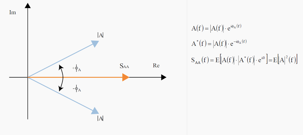
It is computed from the instantaneous spectra of both channels. All other functions are computed during post-processing from the cross-spectrum and the two auto spectrums - all functions are the functions of frequency.

Cross-spectrum

A cross spectrum or cross power spectrum is based on complex instantaneous spectrum A(f) and B(f), the cross-spectrum SAB (from A to B) is defined as:

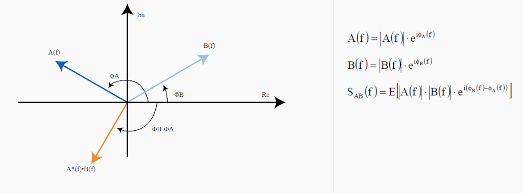
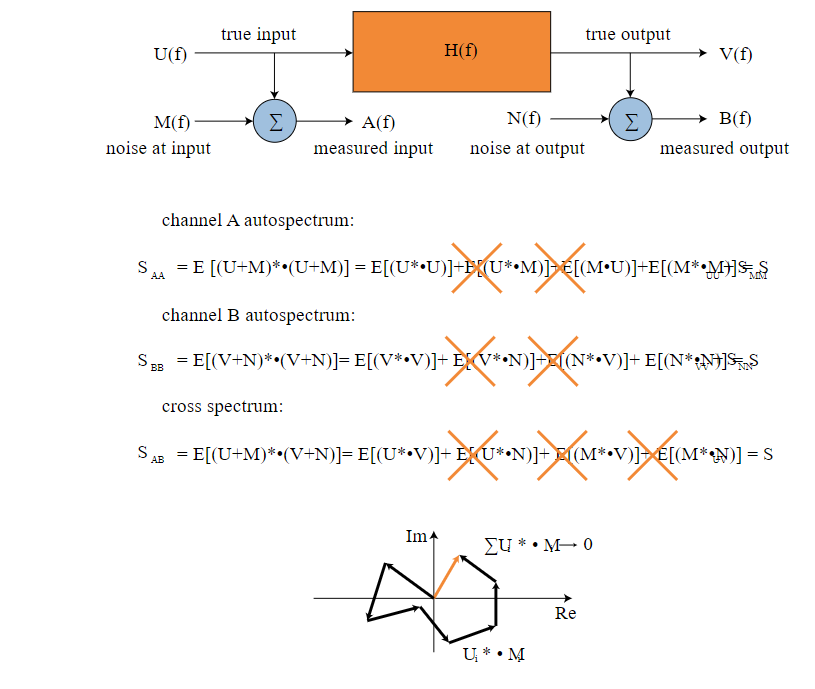
The amplitude of the cross-spectrum SAB is the product of amplitudes, its phase is the difference between both phases (from A to B). Cross spectrum SBA (from B to A) has the same amplitude, but opposite phase. The phase of the cross-spectrum is the phase of the system as well.

The cross-spectrum itself has little importance, but it is used to compute other functions. Its amplitude |GAB| indicates the extent to which the two signals correlate as the function of frequency and phase angle of GAB indicates the phase shift between the two signals as the function of frequency. An advantage of the cross-spectrum is that influence of noise can be reduced by averaging. That is because the phase angle of the noise spectrum takes random values so that the sum of those several random spectra tends to zero. It can be seen that the measured autospectrum is a sum of the true autospectrum and autospectrum of noise, whilst the measured cross-spectrum is equal to only the true cross-spectrum:

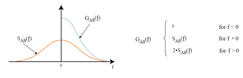
One- and two-sided spectra

Both auto spectra and cross-spectrum can be defined either as two-sided (notation SAA, SBB, SAB, SBA) or as one-sided (notation GAA, GBB, GAB, GBA). One-sided spectrum is obtained from the two-sided one as:

In the image below, we can see a typical FFT screen. The maximum frequency of the FFT is half of the signal sampling frequency (in this case the sample rate was 22000 samples/sec), but in the upper region the results are never reliable, so the sampling result should be set to:

1.25 is the absolute minimum factor for also getting the right values in the upper region of the FFT. A factor of 1.28 is commonly used in signal analysis in order to obtain a 'nice' Analysis Bandwidth (also referred to as Frequency Span). For example having a sample rate given by:

then:

The factor of 2 comes from the famous Nyquist criteria (or more correctly from the Nyquist–Shannon sampling theorem), which says that maximal signal frequency adequately presented in the digitized wave is the half of the sampling rate.

The result of FFT is a set of amplitudes of certain frequencies. The amount of amplitudes in the set is given by the Number of Lines parameter for the FFT. The Number of Lines parameter is user-selectable, and it determines the resolution of the FFT. Line resolution is a change in frequency between two frequency lines, which are extracted from the signal and is calculated with the equation:

So the question is: why not always use the maximum number of available frequency lines, which gives more exact results? The answer is simple: because, with more frequency lines it takes more time to calculate FFT spectra.

Just for fun we can also combine the equations above and we get:

Let's look at the equations above and make a list for the 22 kHz sample rate:

So the number of lines combined with the sample rate also defines the speed of the FFT when non-stationary signals are applied. With more lines, FFT will appear slower and changes in signal will not be shown that rapidly.

Different amplitude scales of FFT can reveal more about the signal if used correctly. Linear amplitude scale gives the best view of maximum peaks in the signal, a logarithmic amplitude scale can show more invisible peaks and signal noise but gives a worse comparison of high and low peaks. Scale in dB gives the best estimation of signal noise if 0 dB is maximum measurable value and is also used in noise measurements, where the dB scaling is actually the result since the human ear has logarithmic sensitivity to noise.

X scale can be either linear or logarithmic. Linear scaling is the correct representation of the mathematic transformation and usually gives the best information for analysis. Sometimes like in the example shown in the picture above it is nice to see the x-axis in logarithmic values since most interesting frequencies are in a lower region. We have to know that just to set the x scale to logarithmic does not enhance the results in the lower region, so the resolution will be better in the upper region since there are more frequency lines available there.

If we use another technique, called CPB (constant percentage bandwidth), also referred to as Octave Analysis, this will give us the same resolution in all regions when the x-axis is logarithmic. This is achieved by the fact that upper region lines cover wider frequency ranges than the lower one.

The resolution of the bands is defined by 1/n description, where n is the number of bands in one octave. The most widely used is the 1/3 octave analysis, which is the standard for noise measurements. 1/12 and even better 1/24 octave analysis already gives good resolution also for signal analysis.

If a sine wave is not located directly on an FFT frequency line, we get amplitude values on both sides of the main band. Such amplitudes can be pretty high and affect FFT results, (with no window function, it can be about 10% of the original values for about 10 neighbor lines). If there is another sine wave in the signal in this region, which is lower than this 10%, it will be completely hidden by the leakage effect.

This is a phenomenon that occurs because the FFT algorithm can only be applied to periodic signals so the sampled input signal is 'periodized'. If the sampled signal is not periodic, or an integer number of periods is not sampled, discontinuities occur in the periodic signal processed by the FFT, causing the energy contained in the signal to 'leak' from the signal frequency bin into adjacent frequency bins. This leakage causes amplitude errors in the frequency spectrum.

As a result of the amplitude errors caused by spectral leakage, small frequency peaks will occur close to larger ones.

Window functions are used to reduce the effects of spectral leakage. Windowing is used to assign a weighting coefficient to each of the input samples, reducing those samples that cause spectral leakage. In effect, samples at the beginning and at the end of the sampling period are reduced to zero so that the discontinuities in the periodized sampled signal are removed.

In the picture below we can see the effect of windowing in a signal.

On the picture below we can see a spectrum of a signal without spectral leakage, spectrum with spectral leakage, and spectrum with windowing.

Windows are characterized by a number of properties as shown in the picture below.

The shape of the window's main lobe is defined by the -3 dB and -6 dB main lobe width. These are defined as the width of the main lobe, in frequency bins, where the window response becomes respectively 3 dB or 6 dB less than the main lobe peak gain. The width of the main lobe of the frequency spectrum is important, as it affects the frequency resolution of the window (ability to distinguish between closely spaced frequency components). As the main lobe narrows, frequency resolution increases. However, with this narrowing of the main lobe, the window energy spreads into the side lobes, increasing the spectral leakage. Therefore, a compromise between frequency resolution and spectral leakage must be reached.

The maximum sidelobe level is defined as the level, in decibels, of the maximum side lobe, relative to the main lobe peak gain.

Sidelobe roll-off rate is the rate of decay of frequency of the side-lobe peaks, in decibels per decade.

The choice of the window depends upon the frequency content of the signal. A popular choice is the Hanning window. This window has quite a narrow main lobe, therefore, good frequency resolution and reasonable side lobe suppression making it suitable for many applications. Blackman-Harris window has excellent sideband rejection with an acceptably narrow main lobe.

The theoretical discrete Fourier transformation (DFT) has absolutely no error. The only problem is that the sum goes from minus infinity to plus infinity. Because we live in a fast-paced world we don't have the time to wait that long so we run into problems.

Amplitude error (picket-fence effect)

FFT results based on FFT time blocks can produce "non-null' results even when the signal does not correspond to the frequencies extracted from the signal, since the pure frequencies are 'leaked' over to neighbor frequencies - a consequence of the finite FFT time block duration T used. For the same reason, if the frequency does not fall exactly on the frequency line, the amplitudes seem to be lower. This is called the "picket fence" effect.

Let's look at the picture below - 10 Hz and 12 Hz are the exact frequency lines. In the example, there are 10 Hz and 12 Hz sine waves marked as black, which are transformed correctly, and there are also frequencies in between which have lower amplitudes. Maximum amplitude error can go up to 35% of the correct value.

For amplitude errors, a bunch of people tried to minimize that problem. Those were Hamming, Hanning, Blackman, Harris, and others. They have created an assortment of functions, which try to correct the errors. Window functions are multiplied with the FFT blocks of the original time-domain signal and since they are usually 0 at the beginning and the end, sine waves could also be in-between lines or phase-shifted and they will leak less over neighbor frequencies - less discontinuity at the FFT block ends.

The picture below shows some of these functions in the time domain.

And here are the most common questions when it comes to FFT: what are the differences between windows and when to use certain windows?

The rule of thumb is that when we want a pure transformation with no window's side effects (for advanced calculations), we should use a Rectangular window (which is equal to no window).

For general-purpose, Hanning or Hamming are commonly used because they provide a good compromise between fall-off and amplitude error (maximum of 15%). This comes from the fact that old frequency analyzers didn't have that many possibilities in terms of frequency lines and these two windows have a narrow sideband.

When a more dynamic range is necessary (we want to see very small signals among large ones), Blackman or Kaiser's window is a better choice because sidebands are 10 times lower than with the Hanning window. However, the sideband width is wider. If more lines in the FFT are chosen, these windows can be used and larger sidebands would still have no real disadvantage.

If correct amplitudes are needed, we should use the flat-top window. The amplitudes would be wrong by only a fraction (as low as 1%). Of course, there is a penalty - neighboring frequencies would also be very high (the sideband width is high). This window is most suitable for calibration. But here it is the same: if a great number of lines are used, then this is often a minor problem.
Just remember that the FFT block length T is the reciprocal of the line spacing, so with more spectral lines it requires a longer time duration per spectrum being calculated. 

Window characteristics (maximum amplitude error, sideband width, highest sideband attenuation, and sideband slope attenuation) are best described in the picture below. We have already discussed the maximum amplitude error: it is an error of amplitude if the sine waves do not fall on the frequency line. Windows try to eliminate this problem and because of that, they widen the first band. The sine waves are no longer on one line in FFT but spread along several lines. The ability to recognize small sine waves among larger ones is determined by the highest sideband attenuation and the sideband slope attenuation. These two values determine the leakage of the FFT and that's nicely seen in the picture below. For example, if there is a signal with a frequency of 30 Hz and an amplitude of 0.0001, we would never see it because the 10.5 Hz signal has bigger leakage than the requested frequency signal. But if the rectangular window is used, we would never even see the signal with an amplitude of 0.01.

For different kinds of windows, the table below shows the values of all window properties. This is a numerical representation of the above-mentioned rules.

The image below shows zoomed FFT of a pure sine wave, which fits the frequency line exactly. Abscissa axis shows the value of the line. In normal FFT, only values of the 0, 1, 2, etc. are calculated, so only those values are shown in the FFT. We can see the width of the first sideband, the highest sideband, and the sideband attenuation very clearly.

If a sine wave signal frequency falls between two lines, we see only the values on each side of the real frequency with sidebands energies that are dependent on the relative frequency deviation between the FFT line and the real frequency. This is best seen if we take a function generator, set the frequency to an exact frequency line, set the amplitude scaling to logarithmic and the FFT will look fantastic. No leakage, exact amplitude. Now switch the frequency from the function generator to the one between two lines in the FFT and the result will be just terrible: large amplitude errors, huge leakage.

There is one more trick with windows: if we are sure that all the frequencies will fall on their frequency lines, a rectangular window will give us the best result. For example to measure the harmonics of the power line (having a fundamental frequency at 50 Hz in Europe), choose 6400 or 9600 sample/sec sampling rate, so that the line resolution will give exact 50, 100, 150 Hz... FFT lines, then choose a rectangular window and observe the perfect result in the Y log scale.

There is another problem arising due to the signal conditioning. As mentioned earlier the sample rate has to be at least twice the maximum signal frequency due to Nyquist–Shannon sampling theorem, else aliasing effects will occur. The image below shows the reason for it. Vertical lines represent samples taken with A/D converter and the black line is the original signal. But if we look at the orange line, which is the signal from the A/D converter, the signal is totally wrong because too few samples per period were taken to correctly represent the signal.

Of course, the problem above is not an FFT problem, but it is very important to know how to correctly identify the cause of the error. And sometimes there are some lines in FFT, which can be only explained in terms of aliasing. In FFT, if we change the frequency to the ranges above the maximum frequency limit, that line will not disappear but will bounce back and will show a fake frequency.

Aliasing example

To see that effect, a function generator and Dewesoft SIRIUS HS (High Speed) set to use no anti-aliasing filter are used, and here the FFT analyzer perfectly shows the problem.

The signal is sampled with 1 kHz.

On the upper left side of the screen, we can see the FFT of the signal recognized by the hardware with no anti-aliasing filter. On the upper right side, there is a picture of a function generator, with the output frequency in the red rectangle.

The first output frequency from a function generator was 400 Hz. Also, the frequency detected by our hardware was 400 Hz.

The second output frequency was 500 Hz (exactly half of our sampling rate). We can see that the hardware with no anti-aliasing filter detects a frequency at 0 Hz (DC). This is because of the described Nyquist theorem.

The third output frequency was 600 Hz. We can clearly see that the signal above 500 Hz bounces back. Our hardware detected a signal with a frequency of 400 Hz.

For the problem of aliasing, there is not much to be done in the FFT domain. Actually, there is absolutely nothing we can do when the samples have already been taken. So the first thing to do would be to choose the A/D board which has anti-aliasing filters in the front, the second thing to do would be to use external filters or we can simply set the sampling rate to more than twice the maximum frequency present in the signal.

To enhance the result, we can use averaging of the signal in the frequency domain. Averaging means that we calculate multiple FFT spectra and average their individual frequency lines.

There are many ways to average the signal, but the most important are Energy (RMS) averaging with Linear or Exponential weighting:

• Energy - is Linear RMS averaging, where each FFT spectrum counts the same in the results, and the result is the square root of the power mean of spectral values.

• Energy (Exp.) - is Exponential RMS averaging - where the FFT spectra are weighted less and less over time, and the result is the square root of the power mean of spectral values. 

Besides these averaging types Dewesoft also supports Maximum hold of spectral values. This Maximum hold type does not actually average spectral values, but instead it keeps individual peak values across multiple spectra. The result is a spectrum of peak line values coming from a mix of spectra. 

Dewesoft also supports an averaging type called Linear, which perform linear but not RMS averaging. This averaging type is rarely used and for most applications the Energy (linear RMS) averaging type would be the correct choice instead.   

There is one more thing about the averaging: loss of information. When averaging is used with window functions, we could lose some data due to the window multiplication effects. In the image below, there is one example where the signal only consists of one pulse. If we average the result, use the window function and if we are unlucky, the signal will fall in the region where the window sets the values to zero, and in the resulting FFT, we will never see this pulse.

Overlapping

That's why there is a procedure called overlapping which overcomes this problem. It no longer calculates averages one after another but takes some part of the time signal, which is already calculated and uses it again for calculation. There could be any number for overlap, but usually, there is 25%, 50%, 66.7%, and 75% overlapping.

50% overlapping means that the calculation will take half of the old data. Now all data will certainly be shown in the resulting FFT.

With 66.7% and higher overlapping, every sample in the time domain will count exactly the same in the frequency domain, so if it's possible, we should use this value for overlapping to get mathematically correct results.

Real-time frequency analyzer

A 'real-time' frequency analyzer is able to calculate and show data with 66.7% overlapping and, therefore, has no data loss.

All signals that are periodic in time but are not pure sine waves, produce base harmonic components as well as additional higher harmonics. The more the signal is not like a pure sinusoid, the greater higher harmonic components become.

A harmonic of a wave is a component frequency of the signal that is an integer multiple of the fundamental frequency f. The harmonics have frequencies 2f, 3f, 4f,... The harmonics have the property that they are all periodic at the fundamental frequency. If the fundamental frequency (first harmonic) is 25 Hz, the frequencies of the next harmonics are 50 Hz (second harmonic), 75 Hz (third harmonic), 100 Hz (fourth harmonic), etc.

1.) Triangle, rectangular

On the left side in the picture below we can see a Triangle signal in the time domain and on the right side is the Triangle signal in the frequency domain.

On the left side in the picture below we can see a Rectangular signal in the time domain, and on the right side is the Rectangular signal in the frequency domain.

2.) Impulse

An impulse is quite an interesting signal - it cannot be described as a sum of sine waves. Or in other words: it is shown equally on all the frequency lines. That's the reason why we use it as the basic excitation principle to get frequency responses of the system. Other common excitation types are swept sine and different types of noise, but this is already part of another story; dual-channel frequency analysis and modal testing.

On the left side in the picture below we can see the Impulse signal in the time domain, and on the right side is the Impulse signal in the frequency domain.

3.) White noise

The theory says that white noise is a signal consisting of all frequencies. That's why the infinite frequency spectrum of white noise is a straight line. The shorter the samples are, the more different amplitudes for certain frequencies we get in the noise level. To get a fixed noise, line averaging must be used. The picture below shows an already averaged FFT of white noise.

On the left side in the picture below we can see White noise in the time domain, and on the right side White noise in the frequency domain.

4.) Beating (two closely spaced signals)

Beating in the time domain is somehow hidden and looks like one frequency with changing amplitudes. Only the FFT will reveal two frequency lines if a high enough line resolution is chosen. The difference between the two frequencies is the modulation frequency shown in the time domain.

On the left side in the picture below we can see a beating signal in a time domain, and on the right side a beating signal in the frequency domain.

5.) Amplitude modulated signal

An amplitude modulated (AM) signal is shown as two sideband frequencies. The difference between the base frequency and the sideband frequency is the modulated frequency (10 Hz in this case) also seen clearly in the time domain. The rule here is the same as with beating - to reveal the modulation; we should choose high enough line resolution. In fact, the time signal or FFT time block, which is the base for the FFT calculation, should show some modulation peaks in order to achieve a proper spectral resolution. When windowing is used the window function will smear the frequency line resolution, such that amplitudes of the sideband frequencies will overlap with the amplitude of the main band frequency if the FFT time block duration T does not cover enough modulation peaks to achieve a sufficient amount of spectral lines between the sidebands and the main band.

On the left side in the picture below we can see an Amplitude modulated signal in the time domain, and on the right side an Amplitude modulated signal in the frequency domain.

FFT preview visual control

There is another option for how to get the FFT of a signal. During the measurement add an FFT preview widget. Click the Design button and then add an FFT preview widget by clicking on the icon.

The FFT preview visual control can display the position and amplitude of maximum peaks, RMS values, or marked peaks.

Difference between FFT analysis module and FFT preview control

How FFTs collect data:

• FFT preview display widget always takes the values left and right in an equal amount from a position of the yellow cursor.

• FFT analysis module takes the values in the block from where you can see the timestamps. The start is on the first stamp and the end is on the second stamp.

The FFT preview is more dynamic and useful to have a quick look wherever you put the yellow cursor, whereas the Math FFT gives you the exact block so you know from where to where some FFT is calculated.

In Dewesoft, we add a new FFT analysis module by selecting the + button and then the FFT Analyser.

When we add a new FFT analysis module the following setup appears:

Output spectra

• Amplitude - outputs FFT Autospectra containing the spectral amplitude values of the signal

• Complex - outputs complex FFT spectra with real and imaginary spectral values of the signal. From the complex data the magnitude and phase of the spectral components can be determined relative to the start of the used FFT time block.

When FFT analyzers are configured, at some point the user must determine how the amplitude of the spectral data should be scaled when it is stored and/or displayed. Dewesoft covers all common types of scaling functions:

• Linear - outputs the same unit as the input signal unit.

• Power - outputs the square of the input signal unit.

• PSD - (Power Spectral Density) outputs the Power divided by the frequency resolution (df_NBW).

• ESD - (Energy Spectral Density) outputs the PSD integrated over the FFT spectral averaging time.

• ASD - (Amplitude Spectral Density) or Linear Spectral Density (LSD) outputs the square root of PSD.

Linear
Linear scaling is normally chosen for stationary, deterministic periodic signals, for example, to analyze the sinusoidal harmonics of rotating machinery. With Linear scaling, periodic sinusoidal signals can be overlaid and compared independently of the selected Line Spacing, since the energy of individual sinusoidal components will (more or less) remain at one spectral line.

Power
Power scaling is chosen for the same reasons as Linear scaling. But while Linear scaling is proportional to the input unit, Power scaling is proportional to the power of the input unit. This has some advantages when inspecting the spectral data, or when using the spectral data for creating derived math channels.

PSD
PSD scaling can be interpreted as the power per frequency and is normally chosen for stationary broadband random signals, for example, to quantify random vibration fatigue.
With PSD scaling, broadband random data can be overlaid and compared independently of the selected Line Spacing in the FFT analyzer, since it takes the Frequency Resolution into account.

ESD
ESD scaling can be interpreted as the energy per frequency and is normally chosen for non-stationary transient signals with finite energy over time, for example, when performing impact measurements.

ASD
ASD scaling is sometimes used for broadband random data having a rather constant spectrum shape since variations in the ASD will be proportional to variations in the input signal level itself.

Amplitude format

After selecting the best-suited Amplitude function for a given measurement scenario, FFT analyzers typically also provide a set of Amplitude formats that specifies how the spectral data should be interpreted. Normally, the relationships among Amplitude formats in FFT analyzers are based on the assumption that spectral lines represent individual sinusoids. Therefore, the following relationships hold:

• Peak - (pk) is the signal positive peak amplitude. 

• RMS - (Root Mean Square) is the signal rms amplitude. For sinusoids, rms relates to the peak value by: 

• Peak-Peak - (pkpk) is the signal minimum-to-maximum peak amplitude. For sinusoids, pkpk relates to the peak value by: 

Frequency weighting

By default the FFT analyzer uses Linear Weighting (no weighting). For sound analysis, acoustic weighting functions can be selected. As opposed to the sound module in math, where the weightings will be calculated in the time domain, this will calculate the sound weighting in the frequency domain.

• Linear weighting (Z) - is linear at all frequencies and it has the same effect on all measured values.

• A weighting - A-weighting is applied to instrument-measured sound levels in an effort to account for the relative loudness perceived by the human ear, as the ear is less sensitive to low audio frequencies.

• B weighting - B-weighting is used for intermediate levels and is similar to A, except for the fact that low-frequency attenuation is a lot less extreme though still significant (-10 dB at 60 Hz). This is the best weighting to use for musical listening purposes.

• C weighting - C-weighting is similar to A and B as far as the high frequencies are concerned. In the low-frequency range, it hardly provides attenuation. This weighting is used for high-level noise.

• D weighting - D-weighting was specifically designed for use when measuring high-level aircraft noise. The large peak in the D-weighting curve is not a feature of the equal-loudness contours but reflects the fact that humans hear random noise differently from pure tones, an effect that is particularly pronounced around6 kHz

Cross-spectrum and reference channel

Cross Power spectra can be calculated when having two or more input channels. By selecting one of the channels as a Reference signal all the selected input channels will be used to calculate cross power spectra. Cross power spectra are calculated as the product of the reference FFT and the FFT from one of the selected input channels. Hereby, if 5 input channels are selected, you will get 5 cross-spectra.

Cross-spectra are complex value channels where the magnitude is the product of the two FFT spectral amplitudes, and the phase is the difference between the two FFT spectral phases.

Window functions

The list of available window functions in Dewesoft is illustrated in the picture above. How to select which window to use was described in the previous section of this training material. 

Resolution settings

 The FFT line resolution can be adjusted by either setting:

• Lines - the number of lines in spectra

• df [Hz] - the line spacing or delta frequency between neighboring lines

• Block duration [s] - the FFT time block length T

All these three settings are related to each other since the number of lines also determines the df which is simultaneously the reciprocal of the block length T.

Averaging

The Averaging Mode determines the duration that the averaged spectra will cover:

• No averaging - outputs individual FFT spectra with no averaging across multiple spectra.

• Block based - outputs FFT spectra that are averaged across a user-defined number of FFT time Blocks (or FFT spectra).

• Overall - outputs one spectrum that are averaged across the entire measurement or the entire selected Recorder time region. 

With the block based averaging, we can average more spectra together by selecting the number of blocks to average together.
Let's say we want to average 2 time blocks of the signal. Each new (averaged) FFT will be calculated every time that the number of spectra are ready to be averaged.

Overall (Averaged) calculation type gives only one averaged FFT spectrum at the end of the measurement. It will average all the blocks in the signal and the output will be only one FFT for the whole measurement.

Overlap

Overlap defines the percentage of the FFT time block that that will be used again for calculation in the next spectrum. Example: 50% overlapping means that the calculation will take half of the old data when calculating the next spectrum. With 50 % overlap the output rate of the spectra will therefore also be twice the rate in comparison to using 0 % overlap.

When a time window function is used, we should use an overlap otherwise some of the data will be ignored as described in a previous section. Therefore, the use of overlap is highly recommended in such cases.

Stop calculation

With the Stop calculation function you can acquire only a selected number of blocks (or seconds) of data. When the condition is reached, the FFT spectrum will stop updating. 

X axis unit

The output x axis can be selected to be described in:

• Hz - periodic cycles per second

• rpm - Rotations Per Minute,  [Hz] * 60.

• cpm - Counts Per Minute, [Hz] * 60. This can be used to indicate cycles per minute that do not relate directly to rotation.

Output quantity and unit

Frequency integration/derivation is possible directly in the FFT analyzer. For example, if the input quantity is acceleration and we select displacement as the Output quantity, the FFT analyzer will preform double integration in the frequency domain. 

The amplitude Output unit can be set relative to the selected output quantity. 

DC cutoff

To remove DC or low-frequency components, select the lower limit of the DC cutoff filter from the drop-down list.

For a measurement example, we used a blue toy with an electromotor and an encoder. An accelerometer was placed on the housing of the toy. When we run the machine up to 3000 RPMs, the machine vibrates.

To observe the behaviour of the machine, we add an FFT analyzer. The input signal is an accelerometer signal that is attached to the rotating machine.

Before we run the machine, let's add a visual control - the 3D graph. Select the Design button and add a 3D graph widget.

The next step is to select the channel that will be shown in the graph. In our example, it was the signal from the FFT analyzer.

The graph shows the amplitude [m/s2] plotted against frequency [Hz]. When we run the machine, we clearly see the first harmonic (values indicated with a red color):

By using the 3D graph widget instead of a 2D graph we can see how the harmonics are evolving over time.

With the 3D graph different types of projections can be selected under the widget properties, as shown below:

Dewesoft supports a long list of helpful and valuable marker types. The full documentation of these markers is described in the processing markers manual, which can be download here: Software Manuals.

The manual can be downloaded as a .pdf file as shown below:

More information can also be found in the online manual for the markers here: Processing Markers Online Manual.

The term Processing Markers is used to indicate that such markers can be used for more than just visual info on graphs. Each processing marker creates a new derived channel that can be used in the setup for additional math operations, and the data can be exported as normally acquired input channels. 

The 2D graph and the 3D graph widgets can display values of the currently selected point with the crosshair cursor.
Let's make a square wave with a frequency of 200 Hz in Dewesoft math and put the signal into the FFT analyzer.

When we go to measure and look at the FFT in a graph widget, we can see that the square wave is composed of a sum of sine waves with different frequencies. We can see those frequencies as peaks in the FFT graph, but now we would like to know the exact position of those peaks.

Free marker

To add markers, right-click on the graph and select Add marker. Under Add marker you find a list of different marker types. Select the Free Marker to add it.

Free markers can be freely added. The marker shows us the frequency of the peak at which it stands and its amplitude.

By pressing the Show marker table in the widget properties, you can see the table of markers - its ID, Group, color, frequency (X-axis), and its amplitude (Y-axis). You can select if you want markers to be visible or not, you can also edit or remove them.

It is possible to open additional settings for the added markers by pressing Edit in the marker table.

Under marker setup for marker types like the Free marker it is possible to enable Improve peak accuracy.

Improve peak accuracy - estimating frequency and amplitude
Depending on the selected window function type used, the frequency component (actual peak) can fall in between two adjacent lines.

In the example below, we have a signal with a frequency of 256.5 Hz and an amplitude of 1. The frequency resolution in our case is 2 Hz. When we add a free marker on the peak (non-interpolated), we see that the marker is at 256 Hz and has an amplitude of 0,97 (because the amplitude is split between two peaks).

If we want to get the exact value, we have to interpolate the peak. To get the right interpolation, at least three lines on each side (left and right) have to have a smaller value than the peak. Now, the frequency of the peak is in the exact position. Also, the amplitude has the right value.

It is possible to estimate the actual frequency and amplitude to a greater resolution than given by the delta frequency (df). Dewesoft uses a weighted average of the values around a detected peak to calculate the exact frequency and amplitude values.

Also, if two or more frequency peaks are within six lines of each other, they contribute to inflating the estimated powers and skewing the actual frequencies. But anyway, if two peaks are that close, they are probably already interfering with one another because of the spectral leakage.

Max marker

The Max marker finds the highest amplitude in the spectrum. Right-click on the FFT graph and select Add marker - Max marker to add such marker types.

When we add Max markers the following setup opens.

The Max marker features the following setup options:

• Current value - shows only a current value of the marker and can be interacted while storing

• Full history - stores calculated values in output channels and can be used as input in other modules

• Improve peak accuracy - if this option is selected the peak position and value are interpolated from the FFT data, as described for the Free marker type.

• Number of peaks - users can manually define the number of peaks in the spectrum they want to find

• Histogram input data - if this option is enabled the marker will find n-highest values in the spectrum. If this option is not enabled, the marker will find n-highest peaks in the spectrum (peak is defined as a values of which the neighborhood bins are smaller than the peak itself)

• Set custom search area - users can define the frequency spectrum in which the peaks are found

Number of peaks
Here we select a number of peaks we want to find. If that number is 1 then the single greatest peak value will be determined, and a derived max channel will be created for that. If the number is set to 3, then it will find also the peak with the second and third-highest amplitude, and three channels will be created. The picture below shows the max marker with 3 number of peaks selected.

RMS marker

RMS marker will sum up all the FFT lines in the selected band and calculates the RMS value. Right-click on the FFT graph and select Add marker - RMS marker to add such marker types.

RMS marker calculates RMS value of the channel between cursors or between defined Positions selected under the RMS marker setup:

The RMS value of the channel between cursors can also be adjusted by dragging cursor with a mouse. RMS will be calculated automatically if the area changes.

Sideband marker

The sideband marker monitors the modulated frequencies to the left and right from the selected centerline.

Let's generate an amplitude modulated signal with a carrier frequency of 1000 Hz and the baseband signal with a frequency of 100 Hz.

Sideband markers have a center marker and several equally spaced sideband markers. By selecting the center marker, you can drag the sideband markers to different positions while still maintaining the individual sideband space.

Each sideband cursor can be selected and moved to a different frequency hence changing the individual ratio of the sidebands with respect to that of the center cursor.

On the FFT, the graph right-click and select Add marker - Sideband marker

The sideband marker draws markers around the selected peak. We have to define the Number of bands (for how many bands in each direction we want to see drawn lines) and Delta (distance between bands in Hz). For example, the selected Position is 1000 Hz, a number of bands are 1, and Delta frequency is 100.

We can see that the central position is at 1000 Hz and we have one band in each direction. So the line on the left side is at 900 Hz and the line on the right side is at 1100 Hz. Distance between the lines can be defined by the user, in our example, it was 100 Hz.

Harmonic marker

The harmonic marker is a great help when identifying the fundamental frequency.

The harmonic marker can be enabled at any frequency. The harmonic marker will mark the harmonics of the selected frequency. The base marker of the harmonic marker can be selected and moved to any other frequency with the harmonics updated live.

Monitoring harmonics is very important in the order tracking analysis. An example was made with a blue toy in the picture below (accelerometer was attached to the machine). We run the machine to 3000 RPMs and measure vibrations in the process.

Move the mouse to the FFT graph, right-click and select Add marker - Harmonic marker to add such a marker type.

We set the First harmonic position at 21.97 Hz.

If we set the Harmonic count to 3, we will see lines at 21.77 Hz, 43.54 Hz (2 x 21.77 Hz), and at 65.31 Hz (3 x 21.77 Hz). And the theoretical harmonics also nicely match our measurement results - the first three harmonics are nicely seen.

You can also pick and drag the fundamental frequency through the FFT spectrum. Harmonics will automatically follow.

Damping marker

Damping markers are best to use in Modal testing when we want to find out how our transfer curve is damped. We select it when we are interested in the quality factor, damping ratio, or attenuation rate of a selected peak.

Move the mouse to the FFT graph, right-click, and select Add marker - Damping maker to add such marker types.

When selecting the damping marker the following setup appears:

Damping factor type can be selected from the following options:

Q factor

The Q (quality) factor of the damped system is defined as:

The higher the Q, the narrower, and 'sharper' the peak is. 

Damping ratio

Damping ratio and quality factor Q are related through the equation: 

Attenuation rate

Attenuation is the gradual loss in intensity of any kind of flux through a medium. It is usually measured in units of decibels per unit length of the medium.

In the picture below we can see a transfer curve of a beam. On each of the peak, we attach a damping factor and in the marker table we can see the Quality factor (Q), which tells us, how much the transfer curve is damped.

If the Damping factor type is chosen as a Damping ratio, the result is Zeta for each peak.

If the Damping factor type is chosen as Attenuation rate, the result is the Attenuation ratio for each peak.

Kinematic markers - bearing cursors

Kinematic markers are used to identify the bearing frequencies and bearing faults.
To use Kinematic markers we have to add Envelope detection math channel.

Each bearing database includes bearing data about the components (cage, rolling element, outer race, and inner race) and at which frequency the components have a peak in the frequency domain.

To add a new bearing go to Kinematic cursor editor.

In the Kinematic cursor editor, add a new bearing or select from the existing database, selecting the Append bearing option.

Channel calculated with Envelope detection math must be now set as the input channel to the FFT analyzer.

At the measurement screen of the FFT analyzer, right-click on the graph and select Add marker - Kinematic marker to add such types of markers.

Now we can see bearing cursors at frequencies that are defined in the bearing database. The table shows to which mechanical part the frequency is related.