

What You’ll Learn 🧰
Understand key filtering concepts: low‑pass, high‑pass, band‑pass, notch (band‑stop), and custom frequency-domain filters
Configure Channel Filters directly in channel setup: set cutoff frequency, filter type, order, and phase (zero/non‑zero)
Apply Math‑based filters, including windowing, moving averages, and FFT domain filtering with IFFT reconstruction
Suppress unwanted signals using digital filters and FFT‑based suppression filters (e.g., remove 50/60 Hz mains hum)
Design and deploy adaptive filters with static or dynamic parameters via formulas or C++ Script
Utilize filter visualizations: preview magnitude/phase response and verify filtering performance in real time
Chain multiple filters and math modules for complex processing—use in workflows like signal smoothing before peak detection or order tracking inputs
Manage filters offline during Analyze mode to compare different processing chains on the same raw data
Course overview
This course provides a comprehensive guide to advanced signal filtering and processing workflows in DewesoftX. The training starts by introducing common filter types—low/high/band-pass and notch filters—and walking through configuring them in the Channel Filters panel. You’ll learn how to choose filter parameters, including cutoff frequencies, order, and phase behavior, and preview the filter’s effect on your signal in real time.
Moving beyond single filters, you’ll explore advanced filtering methods:
Math filters, where signals are transformed in the frequency domain (FFT), processed, and converted back via IFFT—ideal for notch filtering, spectral smoothing, and custom suppression.
Moving-average and windowing filters, to smooth noisy signals before more precise analysis or peak detection.
You’ll also learn to suppress unwanted frequencies—such as powerline interference—using dedicated algorithms with visual validation, and to construct multi-stage filter chains by chaining filters and math modules for complex workflow scenarios.
The course also covers editing filters post‑acquisition in Analyze mode, allowing you to reprocess data with different filter settings without needing to re-record—a powerful tool for iterative data analysis.
By the end of this course, you will be fully equipped to apply sophisticated signal processing chains in DewesoftX, ensuring clean, accurate data for downstream tests like modal analysis, rotor balancing, fatigue testing, and more.
Signal filtering introduction
Let's begin with some terminology, followed by a basic introduction. After that, we will acquaint ourselves with analog and digital filters, as well as converters, and then compare the two. Next, we will look at the different types of filters and their applications. Finally, we will see how to set up and use all of these filters in DewesoftX.
In the field of signal processing, a filter is a device or process that completely or partially suppresses unwanted components or features from a signal. This usually involves removing certain frequencies to eliminate interfering signals and reduce background noise.
Although the function of filters is relatively simple, they are invaluable in modern electronics, particularly in telecommunications.
Terminology


High-pass filter — a filter that allows high frequencies to pass while attenuating low ones.


Band-pass filter — a filter that allows only frequencies within a specific range (band) to pass.


Band-stop filter — a filter that attenuates only the frequencies within a specific range (band).


Notch filter — a filter that rejects a specific frequency (an extreme form of a band-stop filter).
Comb filter — a filter with multiple, regularly spaced, narrow passbands.
All-pass filter — a filter that passes all frequencies but modifies the phase of the output.
Cutoff frequency — the frequency beyond which a filter does not allow a signal to pass.
Roll-off — the rate at which attenuation increases beyond the cutoff frequency; it defines the steepness of the transition between the passband and stopband.
Transition band — the range of frequencies between the passband and the stopband.
Ripple — the maximum amplitude variation of the filter within the passband, measured in dB.
Filter order — the degree of the approximating polynomial; increasing the order sharpens the roll-off and makes the filter response closer to the ideal.
Analog filter
Analog filters are fundamental building blocks of signal processing and are designed to operate on a continuous signal (a signal that has a value at every instant in time). They are electronic circuits whose behavior depends on the elements used:
Passive — made of capacitors, inductors, and sometimes resistors.
Active — use active components such as amplifiers in combination with passive elements.
Filters can be linear or non-linear, depending on the type of equation that describes them. Most analog filters have an infinite impulse response (IIR), meaning that, in theory, the impulse response of the filter never reaches zero. In practical applications, however, the signal gradually approaches zero and can be considered negligible. This occurs because analog circuits consist of resistors, capacitors, and/or inductors, which possess “memory,” preventing their internal states from fully relaxing after an impulse.
Example: A first-order low-pass filter.


Digital filter
A digital filter is a signal processing system that performs mathematical operations on a signal that is:
Sampled — a continuous signal that has been converted into a discrete one.
Discrete-time — unlike a continuous signal, a discrete signal does not have a value at every instant in time; instead, it is quantized.
Digital — a physical signal representing a sequence of discrete values (for example, an arbitrary bit stream or a digitized analog signal).
Digital filters are used in the same way as analog filters: to modify a signal by suppressing unwanted components.
Filter characteristics include:
Type (low-pass, high-pass, band-pass, band-stop)
Cutoff frequency
Order (steepness of the filter response)
FIR or IIR design


A digital filter can have either a Finite Impulse Response (FIR) or an Infinite Impulse Response (IIR):
FIR — the response of the filter to an impulse will reach exactly zero after a finite amount of time.
IIR — occurs when feedback is present in the filter’s topology, causing the impulse response to theoretically never reach zero.
Comparison between continuous and discrete signals:


Comparing analogue and digital filters
Analog filters are much more susceptible to non-linearity (resulting in lower accuracy) because the electronic components used for filtering are inherently imperfect and often have values specified only within a certain tolerance (for example, resistors commonly have a tolerance of ±5%). Their performance can also be affected by temperature and aging. Additionally, circuit elements introduce thermal noise because every component generates heat. As expected, the more complex the circuit, the greater the magnitude of component-related errors. Moreover, analog filters cannot have an FIR response because that would require delay elements.
Where analog filters excel is in high-frequency operation, low latency, and speed. As mentioned in the converter section, a digital filter cannot function without preemptive anti-aliasing, which can only be achieved with a low-pass analog filter. The speed of an analog filter can be 10 to 100 times greater than that of a digital one. It is also worth noting that in very simple cases, an analog filter can be more cost-efficient than its digital counterpart.
Digital filters, on the other hand, excel in areas where analog filters do not. They are more accurate, support both FIR and IIR designs, and can be programmed, which makes them easier to build, test, and adapt. They are also more stable, as they are unaffected by temperature and humidity variations. In terms of cost efficiency, digital filters are generally far superior, especially as filter complexity increases.
The main downside of digital filters is latency, since the signal must pass through two converters and still be processed at high frequencies. In modern electronic systems, both analog and digital filters are often combined to complement each other, achieving maximum speed and accuracy.
Comparison of digital and analog filters:
| Digital filters | Analog filters |
|---|---|
| high accuracy | less accurate due to component tolerances |
| linear phase (FIR filters) | non-linear phase |
| no drift due to component variations | drift due to component variations |
| flexible, adaptive filtering possible | adaption of filters is difficult |
| easy to simulate and design | difficult to simulate and design |
| computation must be completed in the sampling period - limits real-time operations | analog filters required at high frequencies and for an anti-aliasing filter |
| requires high-performance ADC, DAC and DSP | no ADC, DAC or DSP required |
An example of using a filter
Now that you have learned the basics of filters and how they work, we will focus exclusively on digital filters and the different types available, since the main goal of this tutorial is to teach you how to use them in Dewesoft.
The following chapters will demonstrate how to set appropriate filters in Dewesoft, how to apply them, and what their purpose is. But first, let’s look at a simple example that illustrates the use of filters.
Using filters
Why should we use filters in the first place? For this example, I have a tuning fork instrumented with a strain gauge, connected to a Dewesoft SIRIUS measuring device.


When the tuning fork is connected to the STG module, it can be viewed in Measure mode under the Channel Setup screen in the Analog In section.


If you look at the recorder while a static force is applied to the tuning fork, you will notice a change in the signal’s offset.
You can also strike the tuning fork so that it produces a sound at its natural frequency (the conventional way it is used). In this case, you will observe a high-frequency vibration with a gradually decreasing amplitude, caused by air resistance and internal friction within the fork.


If you observe the recorder while a static force is applied to the tuning fork, you will notice a shift in the signal’s offset.
Alternatively, you can strike the tuning fork so that it vibrates at its natural frequency (the conventional way it is used). In this case, you will see a high-frequency vibration with an amplitude that gradually decreases due to air resistance and internal friction within the fork.


This is also an excellent example for learning how to use filters in DewesoftX. Clearly, the signal consists of two components: one in the form of an offset (static load) and another as a dynamic ringing at a 440 Hz frequency.
To extract these two components from the original waveform, you need to apply two filters: a low-pass filter and a high-pass filter.
To do this, add the two filters in the Channel Setup’s Math module.


1. Setting the 1st Filter
Select the input channel, in this case, Tuning Fork.
Leave Design Type set to Preset.
In Design Parameters, confirm that the Prototype is set to Butterworth and set the number of Orders to 6.
Set the Frequencies Filter Type to Low Pass, and update Fc2 to 200 Hz.
This filter will pass all signals below 200 Hz. All frequencies above 200 Hz will be cut off.
2. Setting the 2nd Filter
Select the input channel, again Tuning Fork.
Leave Design Type set to Preset.
In Design Parameters, confirm that the Prototype is set to Butterworth and set the number of Orders to 6.
Set the Frequencies Filter Type to High Pass, and update Fc1 to 200 Hz.
This filter will block all signals below 200 Hz and pass all signals above 200 Hz.
If you display these two filters on the recorder, you will see that the signal is clearly decomposed into the static load and the dynamic ringing. This technique can be used to remove unwanted parts of a signal or to extract specific frequency components from a given signal.


FIR and IIR filters
An FIR filter uses only current and past input digital samples to calculate the current output sample value. It does not rely on past output samples.
The FIR filter works by taking the input channel data and multiplying it by a specific set of coefficients. The simplest example of an FIR filter is the averaging filter. For instance, if we want to average the input data over three samples, the equation would look like this:
The main disadvantage of the FIR filter is that it requires a large number of input points to achieve sharp filtering.


An IIR filter uses the current input sample, as well as past input and output samples, to calculate the current output sample value. The formula can be expressed as follows:
By using the previous output sample, the IIR filter essentially performs exponential averaging. This simple yet efficient formula provides much stronger filtering of the data.


Comparison of FIR and IIR filters:


By the way, these functions were simulated in DewesoftX formulas using the prev and .data functions:
Formula #1


Infinite and finite impulse response
Let's first examine the advantages and disadvantages of the IIR response, then the FIR response, and finally provide a quick summary and overview of both.
The main advantage of IIR filters over FIR filters is their efficient implementation, which allows them to meet specifications for pass-band, stop-band, ripple, and roll-off with a lower filter order compared to a similar FIR filter. This means fewer calculations are needed, resulting in significant computational savings. IIR filters are best used when linear characteristics are not critical and for lower-order filtering applications.
The main disadvantages of IIR filters are instability, feedback, non-linearity, and a limitation in the number of processing cycles.
FIR filters, on the other hand, allow linear characteristics, require no feedback, are inherently stable, and can be easier to design to meet specific frequency response requirements. The disadvantage of FIR filters is that they require more memory and computational power than an IIR filter of similar sharpness or selectivity, especially for lower-order designs.
The following table provides a quick comparison of IIR and FIR filters:
| IIR | FIR |
|---|---|
| impulse response is infinite | impulse response is finite |
| can be unstable | always stable |
| slow | sharp cut-off |
| IIR is recursive | FIR is non-recursive |
| multi-rate signals are not supported by IIR | multi-rate signals are supported in FIR |
| phase response is not linear | phase response is always linear |
| IIR is less accurate | FIR is more accurate |
| IIR transfer function consists of zeros and poles | FIR transfer function consists only of zeros |
| IIR requires less computing power than FIR | FIR requires more computing power that IIR |
| can have limited cycles | no limited cycles |
Setting up filters
Here you will learn how to add a new filter using Dewesoft X.
A new filter can be added within the Dewesoft X Math module by clicking the Add Math button and selecting the appropriate filter from the drop-down menu. You can also use the search bar by simply entering FIR, IIR, or Frequency Domain Filter to quickly find the desired option.
The available filter types are:
IIR Filter (Infinite Impulse Response)
FIR Filter (Finite Impulse Response)
Frequency Domain Filter
IIR filter setup
IIR filters are digital filters with an infinite impulse response, which means that the response to an impulse will remain non-zero over an infinite length of time. They support low-pass, high-pass, band-pass, and band-stop types of filters, as well as multiple input channels. You can choose from Chebyshev, Butterworth, and Bessel filter prototypes. A drawback of IIR filters is that their phase response is not linear.
To add a new IIR filter in the Math section:
In Measure mode, go to Channel Setup and open the Math module.
Search for the IIR Filter tab and open it.
When you select the IIR filter, the IIR Filter Setup window will appear. You can also access this setup window at any time by clicking the Setup button. On the left side of the setup screen, select the input channel to which the filter will be applied. To apply the same filter to multiple channels, simply select all the channels you want to filter.


Within the IIR filter setup, you can choose between two Design Types:
Preset Filter (opened by default)
Manual Filter
IIR filter options
The IIR filter supports high-pass, low-pass, band-pass, and band-stop types of filters.
In the IIR Filter Settings section, you can configure the following options:
Type and Prototype
Order
Cut-off Frequency (Low, High)
Scale
Ripple (only for Chebyshev filters)
You can observe the effects of these settings directly in the Response, Coefficients, and Zeros & Poles tabs for each filter type—Low-pass, High-pass, Band-pass, Band-stop—and for the various prototypes.


Types of Filters:
Low-pass – A low-pass filter attenuates high frequencies in the signal.
High-pass – A high-pass filter attenuates DC and low frequencies.
Band-pass – A band-pass filter attenuates both high and low frequencies, leaving only a specific frequency band.
Band-stop – A band-stop filter attenuates only a specific frequency band, for example, a band around 50 Hz to cancel the effects of supply voltage.
Prototypes of filters:
Butterworth – The Butterworth filter has no ripple and maintains the signal shape with higher orders. The roll-off is defined as (-20 dB/decade) × order. It is also known as a maximally flat magnitude filter, indicating a very flat response in the passband.
Chebyshev I – The Chebyshev filter generally has the steepest roll-off of the three prototypes but introduces ripple in the passband and may not maintain the shape at higher orders. Filter selection often depends on the application.
Bessel – The Bessel filter provides a maximally linear phase response. However, its roll-off is the least steep of the three filter types.
Order
The order of a filter determines its steepness. For a Butterworth filter, the roll-off is (-20 dB/decade) × order. For example, a sixth-order Butterworth filter has a roll-off of -120 dB/decade. This means that if the amplitude at 100 Hz (in the stopband) is 1, the amplitude at 1000 Hz would be 10^(-120/20) = 10^-6.
Higher-order filters require more computational power. In general, six multiplications are needed for every two orders of the filter.
Cut-off frequency
Fc1 (low frequency) – Enter Flow for high-pass, band-pass, and band-stop filters.
Fc2 (high frequency) – Enter Fhigh for low-pass, band-pass, and band-stop filters.
High and low frequency – Enter Fhigh and Flow for band-pass and band-stop filters.
Note: Fc1 must always be lower than Fc2. Filter values are limited by stability. In DewesoftX, filters are calculated in sections, allowing a ratio between cut-off and sampling frequency from 1 to 100,000. This makes it possible, for example, to implement a 1 Hz high-pass filter with a 100 kHz sampling rate.
Ripple
Ripple is the maximum amplitude deviation of the filter in the passband, measured in dB. This option is available only for the Chebyshev filter prototype.
The ripple amplitude of 3 dB results from:
Scale
The scale factor is the final multiplication factor applied before the value is written to an output channel. It allows us to adjust the units of the signal, for example. A good example of using the scale factor is shown in the Integration section.
Digital filter types
This page provides a brief summary of the three different IIR filter prototypes in DewesoftX.
Butterworth
The Butterworth filter is a type of signal processing filter designed to have a maximally flat frequency response—meaning it has no ripples—in the passband and rolls off smoothly toward zero in the stopband. It is also referred to as a maximally flat magnitude filter and provides the smoothest possible response curve of any filter of the same order.


Chebyshev
Chebyshev filters have a steeper roll-off and more ripple in the passband (Type I) or stopband (Type II) compared to Butterworth filters. They are designed to minimize the error between the ideal and actual filter response over the filter's frequency range, but this comes at the cost of ripples in the passband. For some applications, Chebyshev filters with a smoother passband response but a more irregular stopband response are preferred.


Bessel
A Bessel filter is a type of linear filter with a maximally flat group delay (i.e., a maximally linear phase response) across its passband. This linear phase response ensures that passing waveforms are minimally distorted. Bessel filters are often used in audio crossover systems. Analog Bessel filters are characterized by an almost constant group delay throughout the passband, which helps preserve the shape of filtered signals.


Filter prototype comparison
Let's examine an example of a laser output signal with sharp transitions. In the signal, we can observe ringing effects.


The task was to determine the maximum value of the signal.
First, we applied the Butterworth filter prototype (orange). We can see that the filter output exceeds the actual maximum value of the signal, resulting in an incorrect reading.


Next, we applied the Bessel filter prototype (green). Using this filter, we can accurately observe the maximum value of the signal.


FIR and IIR filter comparison
Let's examine a direct comparison between FIR and IIR filters.
For this demo, we use a tuning fork. We connect the fork to the STG module. The fork's natural frequency is approximately 440 Hz, so we set both filters as high-pass filters with a cutoff frequency of 200 Hz.
Excite the fork so that it vibrates at its natural frequency.


When the FIR filter is applied, we can see that there is no phase delay.


When the IIR filter is applied to the signal, a clear phase delay becomes evident.


Response / coefficients / zero & poles preview
At the lower section, you can find useful information about the selected filter. The first element is the Response curve.


The red curve represents the filter’s amplification or attenuation in dB relative to frequency. As a reminder, dB scaling is calculated using the equation:
a[dB]=20⋅log10(A)a[\text{dB}] = 20 \cdot \log_{10}(A)a[dB]=20⋅log10(A)
Thus, the attenuation ratio is calculated as A=10(a/20)A = 10^{(a/20)}A=10(a/20).
For example, if the attenuation is -34 dB, the ratio between the input and output at that frequency is:
A=10−34/20≈0.02A = 10^{-34/20} \approx 0.02A=10−34/20≈0.02
This means that if the input is a 1 V sine wave, the output will be approximately 0.02 V sine wave.
The phase curve (green) indicates the signal delay in degrees.
The lower table displays the filter coefficients used for calculation. The filter is divided into multiple sections for improved stability, with the output of one section feeding into the next. These coefficients can also be copied and pasted using a right-click on the table for use in other calculation programs.


The Zeroes & Poles diagram shows the positions of the filter’s zeroes and poles and provides insight into the filter’s stability.


FIR filter setup
First, add a new FIR filter in the Math section.
In Measure mode, go to Channel Setup and open the Math module. Search for the FIR filter tab and open it.
When you select the FIR filter, the FIR Filter Setup window will appear. On the left side of the setup screen, select the input channel to which the filter will be applied. If you want to apply the same filter to multiple channels, simply select all the channels you want to filter.


A key property of FIR filters is that the phase response is linear. The phase shift in time corresponds to half the number of samples if the filter is calculated using past samples.
Since DewesoftX introduces a calculation delay, we can use a compensation technique to eliminate the filter delay, resulting in no phase shift in both the passband and the transition band. This is a significant advantage compared to IIR filters, which always exhibit some phase shift.
FIR filter settings
For FIR filters, you can set:
Filter type and Window type
Order (number of taps)
Cut-off frequency (Fc1 and Fc2)
Scale
Ripple (only with the Kaiser window type)
You can see the effect of these settings directly in the Response/Coefficients preview for filter types: Low Pass, High Pass, Bandpass, Bandstop, and different Window types.


Filter type
Low Pass – A low-pass filter attenuates high frequencies in the signal.
High Pass – A high-pass filter attenuates DC and low frequencies.
Bandpass – A bandpass filter attenuates high and low frequencies, leaving only a single band of values.
Band Stop – A band-stop filter attenuates a specific range of frequencies.
All-pass – An all-pass filter passes all frequencies with equal gain but alters the phase relationship between different frequencies by varying its phase shift as a function of frequency.
Window type
The window defines the behavior of the filter in the transition band and stopband (the height of sidebands and the width of the main band). Windows are explained in detail in our FFT guide.
Blackman or Kaiser – Suitable when a higher dynamic range is needed (e.g., detecting very small signals among large ones). These windows reduce sideband levels by approximately 10 times compared to the Hanning window, although the main lobe is wider. With more FFT lines, these windows can be used without significant disadvantages.
Rectangular – Best for pure transformations without window-induced effects (useful for advanced calculations). Rectangular window is equivalent to applying no window.
Hamming, Hanning – Common general-purpose windows that provide a good compromise between fall-off and amplitude error (maximum ~15%). Historically used because older frequency analyzers had limited frequency resolution.
Flat Top – Best for accurate amplitude measurements, with errors as low as 1%. The trade-off is wider sidebands, making neighboring frequencies appear higher. Ideal for calibration; modern equipment with high FFT resolution mitigates this issue.
Order
The order of the filter defines the number of coefficients and directly affects the slope of the transition band. Note that FIR filter order is not directly comparable to IIR filter order.
Ripple (only with Kaiser window type)
When a Kaiser window is selected, a Ripple field appears to the right of the Window type field. Here, you can enter the ripple value in dB. This value specifies the maximum allowed passband ripple. Higher ripple values increase passband nonlinearity but make the filter steeper.
Cut-off frequency
The cut-off frequency defines the -6 dB point (half amplitude) of the filter. You can enter cut-off frequencies as follows:
Fc1 (Low frequency) – Use for Low Pass, Bandpass, and Bandstop filters.
Fc2 (High frequency) – Use for High Pass, Bandpass, and Bandstop filters.
Fc1 and Fc2 – Use for Bandpass and Bandstop filters.
Important: Fc1 must always be lower than Fc2. These values are limited by filter stability. In Dewesoft X, filters are calculated in sections, allowing the ratio between cut-off and sample frequency to range from 1 to 100,000. This enables, for example, a 1 Hz high-pass filter with a 100 kHz sampling rate.
Scale
For filters, you can also enter a Scale factor. The scale factor is the final multiplication applied before the output is written to the channel. It allows unit conversion or amplitude adjustment, as needed.
Reduce signal ringing with FIR filter
When acquiring analog data with sharp transitions (such as square waves) using 24-bit Sigma-Delta ADCs (with an anti-aliasing filter), some ringing may be observed. To eliminate or at least smooth this ringing, a FIR filter can be applied.


If you zoom in on the region of the signal at a sharp transition:


For best results, set up the FIR filter as follows:
On the top left under Input, select the channel or channels to which the filter will be applied.
In Design Method, set the number of Taps to 4.
Under Design Parameters, set Windowing to Blackman.
In Frequency Settings, select Low Pass as the filter type, with Fc2 set to 1000 Hz.
After applying the FIR filter, you can see that the ringing has been smoothed:


If you zoom in on the region of ringing and compare the original signal (red) with the smoothed signal (blue), you will notice that the ringing is almost completely gone, and the overall signal shape has improved.


Custom IIR filter
The Custom Defined Filter setup requires:
The number of sections and coefficients.
The Scale Factor, which is the final multiplication factor applied before the value is written to the output channel—for example, it can be used to change the unit.
The values of individual filter coefficients.
An FIR filter consists of a single section because it is stable by definition. IIR filters, on the other hand, can have multiple sections.
You define the number of coefficients per section, which corresponds to the number of rows in the table. This essentially determines the filter order.


The final step is to define the filter coefficients. Enter the a (input) and b (recurrent) values in the z-plane, then press the Update button to apply the filter settings. You can also copy or paste coefficients from the clipboard by right-clicking and selecting either 'Copy to Clipboard' or 'Paste from Clipboard'.

Defining the coefficient
The question now is: how do we define the coefficients? The answer lies in understanding filter design in the s-plane and converting the filter to the z-plane.
Typically, filters are defined in the s-plane. Let's consider a simple example using the general formula for a second-order filter:
To obtain the filter coefficients in the z-plane (time-domain coefficients), the bilinear transformation is used:
where fsf_sfs is the sampling frequency.
This equation highlights an important property of filters defined in the z-plane: they are valid for only a single sampling rate. Therefore, if filters are required for different sampling rates, the coefficients must be recalculated.
By substituting sss in the general second-order filter formula with the bilinear transformation formula, we can obtain the corresponding z-plane coefficients.
The first third of the equation corresponds to the z0z^0z0 coefficient, the second third to z−1z^{-1}z−1, and the final third to z−2z^{-2}z−2. The upper part of the general formula for the second-order filter (with ggg coefficients) represents the input portion, while the lower part (with hhh coefficients) corresponds to the recursive portion of the equation.
If a higher-order filter is required, the equation must be extended similarly, with a larger number of coefficients. The resulting equation will include additional factors, such as z−3z^{-3}z−3, z−4z^{-4}z−4, and so on.
Let’s now consider a simple example of a second-order Butterworth filter. Its prototype in the s-plane is:
where ωc\omega_cωc is the cutoff frequency in rad/s. The cutoff frequency must be adapted to the sampling rate using pre-warping:
By substituting the factors from the general equation, we can derive the coefficients for this filter.
Now, let's create the following filter:
Cutoff frequency: fc=100f_c = 100fc=100 Hz
Sampling rate: fs=1000f_s = 1000fs=1000 Hz
First, perform pre-warping. Pre-warping is used to account for the nonlinearity of the bilinear transformation and to produce a more accurate mapping from the analog filter to the digital filter. The warping effect alters the band edges of the digital filter relative to those of the analog filter in a nonlinear manner.
Next, calculate the coefficients for the direct (input) and recursive parts of the filter by substituting the factors into the equation.
Finally, set the number of coefficients to 3, the number of sections to 1, and enter the 6 calculated values into the table. Press Update. All entered values will be highlighted in red, and the Update button will flash until it is pressed.

")
However, you still need to normalize all the numbers to z0z_0z0 in the bbb (recur.) column. The number in the row z0z_0z0 and column bbb (recur.) must be set to 1. To obtain the correct coefficients, all other numbers in the column must be divided by this particular value.
This means that the actual values will look like this:

")
After entering all the correct coefficients, press the Update button. Once updated, the red highlighting will disappear, and the filter will be ready to use.


Remember, this procedure is valid only for a sampling rate of 1000 Hz. For other sampling rates, you must recalculate the cutoff frequency (fcf_cfc) and the coefficients.
Creating a second-order Butterworth filter is much easier using the DewesoftX standard filters. However, if you require a specific filter, it is necessary to design it manually.
Custom filter import from Matlab
It is possible to import a custom filter from Matlab (registered trademark of MathWorks).
To open the Filter Design & Analysis Tool in Matlab, type fdatool in the Command Window..


After that, the filter design window will appear.


Design the IIR filter in Matlab, then click the Filter Coefficients button. The filter coefficients should appear in SOS matrix form, which is how they are represented in DewesoftX.


In DewesoftX, you cannot enter the scale factors directly, so they must be included in the filter itself. One section in DewesoftX corresponds to one SOS section in Matlab. You need to scale it appropriately: the first three coefficients in Matlab are input coefficients, calculated by multiplying them by the corresponding scale factor. The second three coefficients are recursive coefficients, which can be copied directly into b.
The calculation formulas for a specific section iii are as follows:
| a(input) | b(rekur.) | |
|---|---|---|
| z0 | Scale i * Section i(1) | Section i(4) |
| z-1 | Scale i * Section i(2) | Section i(5) |
| z-2 | Scale i * Section i(3) | Section i(6) |
The coefficients for our example are calculated below:


Response curve / coefficients
For the FIR filter, you can choose between the Response Curve Preview and Coefficients Display.
The red response curve shows the amplitude attenuation of the filter. The amplification ratio is expressed in dB (similar to an IIR filter). The green curve shows the phase delay. In both the passband and the transition band, the phase delay is always zero. In the stopband, the phase angle is not critical due to the high attenuation.


The other display option shows the Coefficients. The upper graph displays the filter coefficients used to convolve the raw data, while the lower graph shows the filter’s response to a step signal.


Filter comparison
Let's examine the difference between an FIR filter and a standard IIR filter. Consider a simple second-order 20 Hz filter with a 1 kHz sampling rate.
The IIR filter is calculated using 6 coefficients, while a comparable FIR filter requires 40 coefficients to achieve the same attenuation. Therefore, the FIR filter is more CPU-intensive for the same performance.
Another point is that while IIR filters can achieve extremely high ratios of cutoff frequency to sample rate (1/100,000 or more), FIR filters are more limited. The achievable ratio increases only with a higher number of coefficients.


Looking at the response graph at 20 Hz (exactly at the cutoff limit):
The green curve represents the original sine wave.
The red curve shows the output of the IIR filter, where the phase delay is clearly visible.
The blue curve shows the FIR filter response, which exhibits no phase shift.
For many applications, it is crucial that signals are not delayed. In such cases, using FIR filters provides a significant advantage.
Frequency domain filter setup
Add a new IIR filter in a math section.
In Measure mode, go to Channel Setup and open the Math module. Then, locate the Frequency Domain Filter tab and open it.
When you add the filter—or press the Setup button on the Frequency Domain Filter line—the setup window will open. On the left side of the setup screen, select the input channel on which the filter will be applied. If you want to apply the same filter to multiple channels, simply select all the channels you want to filter.

Frequency domain filter description
This filter is quite different from other filter types. While IIR and FIR filters operate in the time domain, a frequency domain filter calculates the signal's spectrum using a specific number of lines and overlap, then extracts the RMS value of a selected frequency range. Therefore, the result is not a full spectrum curve but a single value per frequency range.
This filter is useful for extracting low-amplitude peaks in signals that are surrounded by strong harmonics—situations where a traditional IIR filter would struggle to isolate the low-amplitude components.
The example below illustrates an electromotor winding failure, visible as low values at the rotation frequency, even when the line frequency is very high:


Frequency domain filter parameters
To set up the frequency domain filter, it is recommended to observe the signal in the display, choose an appropriate number of lines, select a suitable window type, and then configure the filter parameters.
Frequency domain filter calculation parameters
Number of lines
This defines the resolution of the filter as well as the number of points in the calculation. The resolution must be high enough to clearly extract the desired harmonic but not so high that the result update rate is significantly reduced.
Overlap
Overlap (similar to FFT averaging) specifies how much of the previous data is used in the next calculation. Increasing overlap can improve the result update rate without changing the number of lines.
Window type
The window defines the filter's behavior in the transition and stopbands, including the height of sidebands and the width of the main lobe:
Blackman – Use this when a high dynamic range is required (e.g., to detect a very small signal among large ones). The Blackman window reduces sidebands by a factor of 10 compared to the Hanning window, but the main lobe is wider. With more FFT lines, this wider main lobe is usually not a problem.
Rectangular – For pure transformation with minimal window effects (for advanced calculations), the Rectangular window is used. This is equivalent to applying no window.
Hamming / Hanning – Commonly used for general purposes, providing a good balance between falloff and amplitude error (maximum ~15%). These windows were popular with older frequency analyzers, which had fewer frequency lines and narrow sidebands.
Flat Top – Use when accurate amplitudes are required. Amplitude errors are minimal (as low as 1%), though sidebands of neighboring frequencies are wider. This window is ideal for calibration, and with modern equipment using many lines, sideband width is less of an issue.
RMS amplitude extraction parameters
When the filter type is set to Tracking, RMS amplitude extraction parameters must be defined.
Frequency source
Fixed – The centre frequency remains constant.
Tracking – The centre frequency is determined by a second input channel (e.g., rotation frequency).
Centre frequency
For a fixed frequency source, enter the centre frequency in Hz. This represents the midpoint of the frequency band for amplitude extraction.
Delta frequency
Enter the delta frequency in Hz. This defines the width of the frequency band and depends on the chosen window and number of lines.
If Tracking is selected as the frequency source, additional parameters are required:
Frequency channel
Select the channel that provides the current frequency to be tracked. The unit must be in Hz.
Number of harmonics
Define how many harmonics should be extracted from the spectrum. For example, if 5 harmonics are specified, 5 output channels will be created for each input channel. The first channel corresponds to the centre frequency, the second to twice the input frequency, and so on.
Custom FFT filter
If Custom Filter is selected from the Filter Type, we can design our own filter. This option allows us to create any type of filter curve in the frequency domain and calculate the RMS value. Sometimes it is difficult to define filter characteristics in the time domain, but they may already be defined in the frequency domain. The Custom FFT Filter is ideal for such cases.


If the frequency source is external, we can specify the channel that provides the frequency. The filter will then automatically adjust its characteristics to ensure correct filtering, similar to the time-domain response. This feature is particularly useful, for example, in CA noise calculations using an external clock.
Derivation
Mathematical operations such as differentiation and integration are also types of filters. Differentiation acts like a high-pass filter, while integration behaves like a low-pass filter and can also filter the DC component.
Derivation
The derivative of a function of a real variable measures the sensitivity of a quantity (the dependent variable) to changes in another quantity (the independent variable).
For example, the derivative of the position of a moving object with respect to time is the object's velocity. This indicates how quickly the object's position changes as time progresses.
Geometrically, the derivative of a function can be interpreted as the slope of the curve of the mathematical function f(x)f(x)f(x) plotted against xxx. However, its significance extends beyond this simple geometric interpretation. Many physical quantities, such as velocity, acceleration, and force, are defined as instantaneous rates of change of another quantity. The derivative provides a precise instantaneous value for that rate of change, enabling accurate modeling of the desired quantity.
The derivative of the function f(x)f(x)f(x) evaluated at x=ax = ax=a gives the slope of the curve at that point.


Double derivation
The second derivative of a function fff is the derivative of the derivative of fff. It measures how the rate of change of a quantity itself changes.
For example, the second derivative of the position of a vehicle with respect to time is the vehicle's instantaneous acceleration — the rate at which its velocity changes over time.
Integration
The integral of the function f(x)f(x)f(x) over the range x=bx = bx=b to x=cx = cx=c gives the area under the curve between these points.


Geometrically, the integral represents the area under the curve of the function f(x)f(x)f(x) plotted against xxx. Integration provides a mathematical way to sum an infinite number of infinitesimally small blocks to obtain a precise analytical expression for the total area.
This is crucial in geometry and profoundly important in the physical sciences, where many physical quantities can be represented as the area under a curve. For instance, the area of a small strip under the curve can be interpreted as its width multiplied by its height.
For example, finding the center of mass of a continuous body requires weighting each element of mass by its distance from an axis of rotation. Integration is necessary to calculate an exact value. Many physical problems involve such infinite sums, making the integral an essential tool for scientists and engineers.
Double integration
Double integration is particularly useful for calculating displacement from acceleration and is therefore commonly applied to dynamic signals.
Derivation and double derivation
Add a new Integral / Derivative math line in the Math module.
In Measure mode, go to Channel Setup and open the Math module. Search for the Integral / Derivative tab and open it.
Differentiation and double differentiation are used, as the name suggests, to calculate the derivative of the chosen input signals. The application range is not divided into separate areas, as the procedure is similar in all cases. The basic calculation is simple: subtract the previous value from the current value and divide by the time interval.
Derivation setup
However, this calculation can produce very noisy signals, especially at high sampling frequencies. You can observe the derivative of a 20 dB/decade rising filter in the frequency domain. Sometimes it is useful to remove high-frequency components.
You can enable the option Filter High Frequencies and configure the filter by choosing:
Order – at least 2 for single derivation and at least 3 for double derivation
High Cutoff Frequency – the maximum frequency to allow in the signal
For example, when calculating acceleration from vehicle speed, a car cannot physically accelerate at frequencies higher than approximately 10 Hz; higher frequencies are usually just vibrations. With this in mind, you can set the High Frequency to 10 Hz to capture the real vehicle acceleration.
Scale Factor
The scaling factor is handled as follows: for derivation, the input is divided by seconds, and for double derivation, it is divided by seconds squared.
For example:
km/hour/sec=1000 m3600 sec/sec=0.278 m/s²=0.2789.81 g≈0.0283 g\text{km/hour/sec} = \frac{1000 \text{ m}}{3600 \text{ sec/sec}} = 0.278 \text{ m/s²} = \frac{0.278}{9.81} \text{ g} \approx 0.0283 \text{ g}km/hour/sec=3600 sec/sec1000 m=0.278 m/s²=9.810.278 g≈0.0283 g
You must enable "Use Custom Scale" and enter this value in the scale field to obtain correct results.
Integration
There are two main purposes of integration: the first is to calculate quantities such as traveled distance from a measured velocity or energy from measured power. The second is to calculate vibration velocity from measured acceleration.
A clear difference between these two applications is that, in the first, the carrier of information is the DC value—the offset (traveled distance or consumed energy). In the second application, the offset represents only measurement error, while the carrier of information is the dynamic part of the signal, such as vibration velocity.
For operations such as integration and differentiation, you must add the Integral / Derivative line from the Add Math module.
Integrating Distance from Velocity
Suppose you have velocity in km/h as the input channel. Select it and switch OFF the option Filter Low Frequencies and DC. The next step is to define the Scale, keeping in mind that integration adds a time unit (sec) to the measurement.
Example:
If the input is in km/h:
km/h×sec=1000 m3600 sec×sec=0.278 m\text{km/h} \times \text{sec} = \frac{1000 \text{ m}}{3600 \text{ sec}} \times \text{sec} = 0.278 \text{ m}km/h×sec=3600 sec1000 m×sec=0.278 m
To obtain the output in meters, enter 0.278 as the scale factor.
To obtain the output in kilometers, enter 0.000278.
Another example: if the input channel is power in kW:
kW×sec=kW×13600 h=0.000278 kWh\text{kW} \times \text{sec} = \text{kW} \times \frac{1}{3600} \text{ h} = 0.000278 \text{ kWh}kW×sec=kW×36001 h=0.000278 kWh
This is the scaling factor for the calculation.
Integrating Dynamic Signals
When integrating dynamic signals, such as vibration acceleration, the measured signal often contains an offset due to the amplifier and ADC. This offset can cause unwanted drift in the integrated result. To prevent this, enable the option Filter Low Frequencies and DC to remove the offset.


Next, you need to define the Order. Be aware that integration is equivalent to a filter of order 1, so to effectively remove DC values, you should choose a high-pass filter of order 2 or higher. The Low parameter determines the frequency at which the resulting velocity will be cut off.
High values of Low (e.g., 10 Hz) will result in very fast stabilization in the case of overload, but they may also remove important signal information.
Low values (<1 Hz) will result in slower stabilization times (typically 50–100 seconds for a 1 Hz filter) but will allow virtually the entire frequency range to pass.
For vibration measurements, a typical Low value ranges from 3 to 10 Hz for general-purpose applications. For low-frequency vibrations, such as those from the human body or building movement, values between 0.3 and 1 Hz are used. For specialized applications, like monitoring seasickness or very tall structures (e.g., TV towers or cranes) that move at extremely low frequencies, values between 0.1 and 0.3 Hz may be necessary. Keep in mind that stabilization in these cases will take a long time. Additionally, ensure that your sensors can accurately measure such low-frequency signals. General-purpose ICP sensors typically have a cutoff frequency between 0.3 and 1 Hz, making them unsuitable for these specialized low-frequency applications.
Scale – Scaling Factor
Now, consider the Scale factor for this application. Assume that you measure acceleration in g. If you want the output in mm/s, you need the following scaling factor:
1 g×sec=9.81 m/sec²×sec=9.81 m/s=9810 mm/s1\text{ g} \times \text{sec} = 9.81 \text{ m/sec²} \times \text{sec} = 9.81 \text{ m/s} = 9810 \text{ mm/s}1 g×sec=9.81 m/sec²×sec=9.81 m/s=9810 mm/s
Therefore, enter 9810 in the scaling field to obtain correct results.
Output unit
For output signal from your filter, you can choose from already defined units, if the measured physical quantity is correctly set up.
m/s
mm/s
km/h
mph
knot
ips
Double integration
Double integration is mainly used to directly calculate displacement from acceleration, so it is typically applied to dynamic signals. Your output unit will be multiplied by sec². Therefore, you need to enable the option to Filter low frequencies and DC. However, take care: since double integration is equivalent to a second-order filter, you should choose an order of 3 or higher for the low-frequency filter.
Calculating the Scale – Scaling Factor
Usually, you want the measurement result in μm (micrometers). Therefore, you need to enter the appropriate scaling factor:
Practical example of integration and double integration
Let’s consider an example using an accelerometer on a shaker, recorded with a high-speed camera.
The green trace represents the signal from the accelerometer, red represents velocity, and blue represents displacement.
Velocity Setup (Integration)
Operation: Integration
Filtered low frequencies and DC: Enabled
Order: 2, with Low set to 4 Hz
Output unit: mm/s
Displacement Setup (Double Integration)
Operation: Double Integration
Filtered low frequencies and DC: Enabled
Order: 4, with Low set to 4 Hz
Output unit: mm
The accelerometer at the top position shows that the calculated displacement is consistent with the actual position measured by the camera.

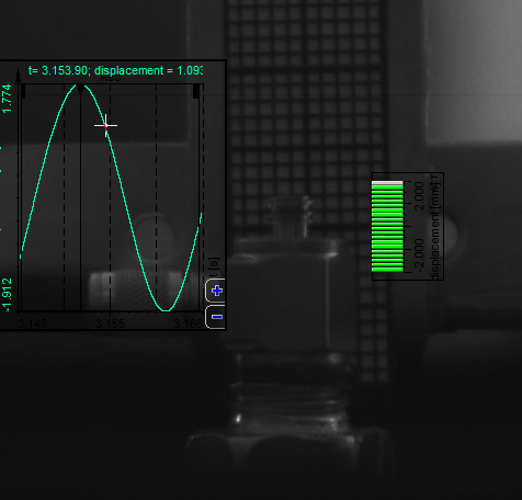
The accelerometer at the middle position shows that the calculated displacement is consistent with the actual position measured by the camera.


Because integration and derivation are types of IIR filters, a phase delay occurs between the signals.


The following example demonstrates how to measure the phase delay between signals. You need to use a mathematical operation called Correlation (add it under the Math section) to calculate the cross-correlation between two signals

Add a 2D graph and apply it to the cross-correlation. Select the Complex presentation as Phase (°). Zoom in to determine the phase at the shaker’s frequency (in this case, 50 Hz). According to theory, the phase shift should be 90°.


Page 1 of 28