Combustion Engine Analysis and Setup in DewesoftX

Course overview

This course provides a deep dive into engines’ thermodynamic and dynamic behaviors using DewesoftX. You’ll start by covering the fundamentals: piston-driven energy conversion, differences between spark-ignition and diesel cycles, and how the CEA module integrates engine data acquisition—combining cylinder pressure and crank-angle information to derive combustion metrics.

Through practical setup lessons, you’ll configure analog pressure channels and high-resolution angle sensors (e.g., encoder, CDM), then set up the CEA plugin. This includes entering cylinder count, stroke type, stroke geometry, and ignition timing. You’ll apply signal filtering and mapping functions to align measurements accurately across engine cycles.

Next, the training focuses on result calculations: extracting peak pressures, crank-angle positions of pressure peaks, heat-release curves, and polytropic coefficients. You’ll also learn how to detect knocking events using a high-pass filter (5–12 kHz) and knock-factor logic, which helps differentiate true knock from background noise by comparing filtered signals within reference and knock-specific angle windows.

Advanced modules cover combustion noise analysis—converting spike-filtered pressure to sound-level metrics—and the use of statistical functions for cycle-by-cycle trend monitoring and optimizing engine performance. You’ll practice exporting results, including P–V plots, heat-release data, TDC offsets, and knock logs. Finally, the course shows how to integrate CEA data with other Dewesoft modules—like CAN bus, video sync, GPS, and ECU data—for a complete engine test setup.

By the end of the course, you’ll be able to accurately acquire, analyze, and interpret combustion data with DewesoftX—improving engine design, optimizing performance, and diagnosing combustion-related issues.

High-accuracy combustion analyzer system from Dewesoft is used for engine research, development and optimization and testing of ignition systems, exhaust systems, and valve control gear.

Internal combustion means just what it says: that fuel is burned inside the engine. In a car engine, gasoline is burned inside the engine, which ignites the fuel and releases energy that moves the car. There are also other methods of internal combustion, such as diesel engines and gas turbine engines. Internal combustion is an efficient system that requires a relatively small engine to create motion. It is also more fuel-efficient than external combustion engines, such as an old-fashioned steam engine.

Gasoline engines used to be as inefficient as steam engines. In 1876 the gasoline engine was invented and it was no more efficient than the steam engine, which used external combustion. A lot of fuel was wasted. In 1878, Rudolph Diesel decided to develop an engine with higher efficiency, and in 1892 the diesel engine was born. It was more efficient as an internal combustion engine, but it took many more years to develop a diesel engine that was cleaner and quieter. Early diesel engines spewed out sooty smoke and at first were only used in trucks. Today, new advancements in this method of internal combustion have improved the diesel engine. The difference between gas and diesel engines is the way fuel is converted to energy.

Turbines are another method used to create power with a spinning motion. There are wind turbines, steam turbines, water turbines, and also gas turbines. Gas turbines work on the principle of internal combustion. In a modern gas turbine engine, the engine produces its own pressurized gas by burning fuel. The engine can burn propane, natural gas, kerosene, or jet fuel. The burning fuel creates heat, the heat, in turn, expands the air, and a high- speed blast of hot air spins the turbine.

An internal combustion engine (ICE) is a heat engine where the combustion of a fuel occurs with an oxidizer (usually air) in a combustion chamber that is an integral part of the working fluid flow circuit. In an internal combustion engine the expansion of the high-temperature and high-pressure gases produced by combustion applies direct force to some component of the engine. The force is applied typically to pistons, turbine blades, rotor, or a nozzle. This force moves the component over a distance, transforming chemical energy into useful mechanical energy.

The first commercially successful internal combustion engine was created by Etienne Lenoir around 1859 and the first modern internal combustion engine was created in 1876 by Nikolaus Otto.

The term internal combustion engine usually refers to an engine in which combustion is intermittent, such as the more familiar four-stroke and two-stroke piston engines, along with variants, such as the six-stroke piston engine and the Wankel rotary engine. A second class of internal combustion engines use continuous combustion: gas turbines, jet engines and most rocket engines, each of which are internal combustion engines on the same principle as previously described. Firearms are also a form of internal combustion engine.

In contrast, in external combustion engines, such as steam or Stirling engines, energy is delivered to a working fluid not consisting of, mixed with, or contaminated by combustion products. Working fluids can be air, hot water, pressurized water or even liquid sodium, heated in a boiler. ICEs are usually powered by energy-dense fuels such as gasoline or diesel, liquids derived from fossil fuels. While there are many stationary applications, most ICEs are used in mobile applications and are the dominant power supply for vehicles such as cars, aircraft, and boats.

Typically an ICE is fed with fossil fuels like natural gas or petroleum products such as gasoline, diesel fuel or fuel oil. There is a growing usage of renewable fuels like biodiesel for compression ignition engines and bioethanol or methanol for spark-ignition engines. Hydrogen is sometimes used, and can be obtained from either fossil fuels or renewable energy.

Diagram showing the operation of a 4-stroke spark-ignited engine. Labels: 1 - Induction, 2 - Compression, 3 - Power, 4 - Exhaust

1. Intake, induction or suction: The intake valves are open as a result of the cam lobe pressing down on the valve stem. The piston moves downward increasing the volume of the combustion chamber and allowing air to enter in the case of a compression ignited (CI) engine or an air-fuel mix in the case of spark-ignited (SI) engines that do not use direct injection. The air or air-fuel mixture is called the charge in any case.

2. Compression: In this stroke, both valves are closed and the piston moves upward reducing the combustion chamber volume which reaches its minimum when the piston is at TDC. The piston performs work on the charge as it is being compressed; as a result its pressure, temperature, and density increase; an approximation to this behavior is provided by the ideal gas law. Just before the piston reaches TDC, ignition begins. In the case of a SI engine, the spark plug receives a high voltage pulse that generates the spark which gives it its name and ignites the charge. In the case of a CI engine the fuel injector quickly injects fuel into the combustion chamber as a spray; the fuel ignites due to the high temperature.

3. Power or working stroke: The pressure of the combustion gases pushes the piston downward, generating more work than is required to compress the charge. Complementary to the compression stroke, the combustion gases expand and as a result their temperature, pressure, and density decreases. When the piston is near to BDC the exhaust valve opens. The combustion gases expand irreversibly due to the leftover pressure - in excess of back pressure, the gauge pressure on the exhaust port; this is called the blow-down.

4. Exhaust: The exhaust valve remains open while the piston moves upward expelling the combustion gases. For naturally aspirated engines a small part of the combustion gases may remain in the cylinder during normal operation because the piston does not close the combustion chamber completely; these gases dissolve in the next charge. At the end of this stroke, the exhaust valve closes, the intake valve opens, and the sequence repeats in the next cycle. The intake valve may open before the exhaust valve closes to allow better scavenging.

The DewesoftX Combustion analysis math module enables the Analysis of internal combustion engines. If we measure the pressure inside the cylinder and the angle of the shaft, we can calculate the main indication values for engine development and testing, like maximum pressure, position of maximum pressure, heat release, knocking, and other important parameters.

The combustion analysis is fully integrated inside the Dewesoft X software, which means that we can use any functionality of Dewesoft including CAN bus, video, other analog signal acquisition, and more.

The video below shows how easy and fast it is to setup combustion analysis in Dewesoft and start measuring.

SIRIUS Combustion Analyser data acquisition systems are used for engine research, development, and optimization. They are also used for component development and testing such as ignition systems, exhaust systems, and valve control gear. The system consists of our top of the notch isolated SIRIUSi hardware and the well-known DewesoftX software package for measurement and analysis.

It supports angle and time-based measurement results and uses highly sophisticated algorithms for online or offline mathematical and statistical calculations of heat release and other thermodynamic parameters.

The combustion analyzer can be fully integrated within a testbed and also supports data from other sources: e.g. Video, CAN, Ethernet,... . If the powerful integrated post-processing features of DewesoftX are not enough, you can even export the data to several different file formats.

In addition to combustion analysis, the system can be expanded to handle other measurement applications such as hybrid testing on the power train, noise, and vibration measurement together with synchronized video or GPS data.

DAQ system overview

Pressure sensor(s) are used to measure the cylinder pressure of the engine. Depending on the sensor type, these can be directly connected to our SIRIUSi amplifier like any other input channel or through external signal conditioning amplifiers. Charge type sensors can be connected to CHG amplifiers directly.

Additionally an angle sensor is needed for getting angle domain measurement results. Several different types are supported by the Dewesoft Combustion Analyser. Additional mounted CDM (Crank Disc Marker) sensors or digital native CDM sensors (like 60-2 or 37-1,...) with TTL outputs can be connected to dedicated counter inputs.

Sensors with analog output can:

• be directly connected to analog input channels,

• or to counter inputs via the DS-TACHO device.

In both cases, the DewesoftX re-sampling technology gives you an angle resolution down to 0.1°.

Like many other modules, Combustion Engine Analysis is also an option to the standard DewesoftX package. Simply in the Channel setup tab press More and select the Combustion engine analysis to add the module.

The basic settings for the CEA module need to be done here as well. Before you add the module you can click on the screwdriver icon on the right of the Combustion engine analysis option to enter the CEA settings, or if you have already added the module, simply open the general Settings, select Extensions tab and find CEA module in the tree window. CEA settings are previewed on Image 5.

CEA Settings:

• The settings for the encoder limit - Check encoder pulses are only used in real angle domain acquisition and therefore not needed for the Dewesoft's Combustion Engine Analyzer.

• If Scope mode is enabled, CEA skips cycles - in other words it does not calculate all cycles. There are several levels of scope mode available. Depending on this setting, the CEA-module also skips calculations depending on the measure mode (storing, not storing, trigger,...). 

  • The default setting which should be used for CEA to calculate, store and visualize all cycles is: never 

• Engine templates (eg. Calculation methods) are stored in the engine templates path.

• Limit the maximum number of cylinders on generated display is related only to the preview of an automatically generated measuring display.

The combustion engine analyzer inside DewesoftX is just one out of several other applications modules that offers dedicated mathematics and dedicated visual controls like the p-V diagram or the CEA scope.

Since the analog channels of the Sirius system are the input for the mathematics calculations, you must first set up the amplifier and configure the scaling of the physical unit. This is done in the Analog section of the setup screen.

When you are satisfied with the Analog configuration you can go to the next step and use those analog channels as input for the CEA module. 

You can use the same analog input channels that you have used in the Combustion Engine Analyzer module for any other mathematics or applications (e.g. FFT, etc.) in parallel! This gives you a multi-functional instrument suitable for nearly any application. moreover, output channels from one mathematics module can be used as input channels for any other module.

When connecting sensors for combustion engine analysis, extreme caution should be made while selecting the correct filters.

Correct hardware should be selected for the type of application (engine) that will be used. If it is going to be a very low-RPM engine and charge type pressure sensors will be used, then a Sirius device with charge inputs should be used. Otherwise also DSI-CHG adapters are possible, but they do not have the same filter settings as charge inputs. On the images above a clear difference can be seen for the lowest High-pass filter setting on a SIRIUS with CHG inputs (Image 9) and a DEWE-43 with DSI-CHG-50 adapter (Image 8).

Signal noise should always be reduced as much as possible with quality cabling and correct mounting of the pressure sensor. If there is still unwanted noise in the pressure signal, then filtering can be used to eliminate this.

High-pass filter

For a low-RPM engine, the high-pass filter shouldn't be set too high.

Low-pass filter

For a high-RPM engine, the low-pass filter shouldn't be set too low.

You must configure the Combustion Engine Analyzer module after setting up the analog input channels.

The configuration of the CEA module is split into 3 sections:

• Engine settings: Defines the geometry of an engine and assigns the channels to the cylinders

• Encoder settings: Assign the encoder/angle sensor, resolution and the TDC detection

• Result definition: Enables/disables different possible calculations and the output channels for the CEA module 

Engine settings are defined by four major fields inside the CEA module as it is shown on image 13: Basic parameters, Volume per cylinder, Selected cylinder settings, and Cylinder overview.

Basic parameters

Volume per cylinder

In the field Volume per cylinder the Volume source first needs to be defined. This will define the geometry of a cylinder which can be in fact:

• written in manually - Geometry option,

• imported curve as a Text file or 

• defined within the selected Engine template.

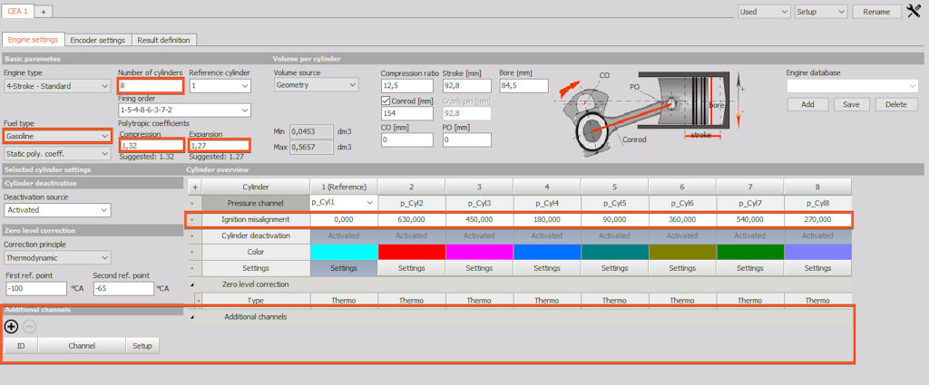
Selected cylinder settings

For each cylinder Selected cylinder settings can be applied, where Cylinder deactivation, Zero level correction, and Additional channels can be set. This is done by clicking the Settings button in the Cylinder overview for the desired cylinder as it is shown in image 18.

Zero level correction

Dewesoft CEA supports three different correction principles:

Additional channels

Additional channels can be applied to each cylinder. These channels are aligned with the corresponding cylinder and will be available in the CEA-Scope diagram, and are as well as the pressure channels recalculated to an angle domain. As an example, you can also apply the Injection or Ignition signal in order to display it together with the pressure signal.

Signals for additional channels do not need to be only the analog signals, but can be also output from other modules, for example, torsional vibration outputs can be added to CEA to view the results in the angle domain of the engine. 

For example, if an injection signal is applied and the Number of injections (events) is set to 3, the trigger level for start trigger is set to 2V, and the end trigger level is set to 1V, the each time the ignition signal crosses 2V it will return the angle position, related to the cylinder where it is applied [deg]. The same is true for the end of event: if the signal crosses 1V (neg. edge) the position will be returned [deg].

In a real measurement, you can set trigger level values based on easy pre-measurement - simply start the measurement in Measure mode and observe the signal values for each injection channel. Then return to CEA set up and rewrite those values in trigger level fields.

Cylinder overview

For each cylinder the corresponding pressure channel needs to be assigned from the channel input list. Also the ignition misalignment relative to the reference cylinder needs to be entered in degrees.

The sampling type of the Dewesoft CEA is always a time domain. This has the advantage that all time-domain related functions are not influenced by changes in the sample rate due to shaft speed, and will stay the same. For example a power calculation is only working in the time domain (fixed sampling rate). Of course CEA is still calculated in angle domain, so the CEA time-domain data are always recalculated into the angle domain.

The required high calculation power for recalculating time-based signals into angle based is spread over all available CPU cores of your PC.

Angle sensor setup is done in the Encoder settings tab as it is shown on the image 22.

Sensor types and angle resolution

Nearly any angle sensor type is supported. For getting the relation to a fixed angle position the sensor must support a fixed angle mark. The drop-down list will automatically show all suitable sensor types from the counter database as it is shown in image 23.

To add a new counter sensor click Options -> Editors -> Counter sensors and you will enter the Counter sensors editor as it is shown on the image below.

After the sensor type is selected, we need to define where the sensor is connected to.

Under properties, the fine adjustment for the angle sensor must be done. In the case of analog sensor selection, the trigger levels can be precisely adjusted. First the trigger edge is defined, according to the signal. Also trigger and retrigger level is set. It is recommended to use the retrigger level to avoid false triggers. False triggers will disturb the CEA operation, and cause incorrect angle information.

Retrigger: After a trigger occurs, the retrigger level must be crossed, so that the trigger is armed again. Thus noise around a trigger will not cause any false triggers.

If a digital sensor is selected, the property will open the counter channel setup of the sensor. This is convenient, because you can define the trigger: e.g. you can invert the signal input or apply an input filter to avoid double triggering.

The next step is to define the target angle resolution for the combustion analysis mathematics. The Upper frequency is limited by the selected resolution and the dynamic acquisition rate in the Analog channel setup.

Take care of this limit to avoid aliasing effects by the re-sampling algorithm. As a Resampling type, an unfiltered method can be selected which is a linear interpolation from the time to the angle domain. The filtered type is based on an FIR polyphase decimator with a filter frequency of angle resolution * 2 to avoid aliasing effects in the angle domain data.

TDC detection

Top dead center detection is used to shift the reference cylinder pressure to 0 deg. The offset between angle sensor zero and the TDC position of the reference cylinder is called the trigger offset. This can be entered manually, or it can be measured.

Image 29 shows the angle offset of a not fired engine (cranked).

For automatic TDC detection (Start button), the no of cycles has to be entered. CA will measure the average offset of the set of cycles automatically. The Maximum pressure will appear before the real TDC of the piston, which is caused by thermodynamic losses and blow-by. That's why the measured value is corrected with the thermodynamic loss angle.

After TDC detection is finished, the average value (which includes the Thermodynamic Loss angle) will be set automatically for the trigger offset.

The example above was using the installed pressure sensor to measure the TDC. This is a very convenient and fast way of doing it. The only variable is the thermodynamic loss angle.

Instead of a pressure sensor, a TDC sensor can be used. The TDC sensor must be connected to an analog input and assigned to the reference cylinder in the CEA setup. The thermodynamic loss angle must be set to 0, and the automatic TDC detection can then be started again. After the measurement, the pressure channel must be set in the CA setup.

There are plenty of options that can be used when it comes to the Result definition for CEA inside Dewesoft X as it is shown in image 32. Detailed channel list overview and their description is available in the Combustion analyzer manual, chapter 7.3. Channel overview on page 25.

For every Group name - Acquired signal and Standard calculations, different values can be used for calculation and different types of averaging can be enabled:

In Result definition from the previous chapter 'How to define the Results?' it was seen that there are plenty of different calculations that can be applied as a result. The following section will introduce all the calculations that can be used inside Dewesoft X.

The Group name column from the image 32 in Result definition tab is divided into three groups: 

• Acquired signals, which are by default selected as 'used' for calculation

• Standard calculations that are totally optional for result definition.

• Two stroke calculations that are available only when two stroke engine is selected in engine settings.

There are two types of thermodynamics calculations that can be used. 

Thermodynamics 1 is the basic thermodynamic calculation that was implemented in the first CEA module and it was available in previous versions of Dewesoft X. Now it is basically only used for a relevant comparison in case you obtain some older results. While Thermodynamics 2 is an upgraded and advanced thermodynamic calculation algorithm that is now used as a primary tool for such calculations in Dewesoft X. 

Thermodynamics 2 and Temperature calculation are closely related, so when clicking on Thermodynamics 2 Setup button, the settings for temperature calculation will also pop-up as it is shown on image 37. 

There are a few settings that can be defined in Thermodynamics 2 and Temperature result definition: 

• Thermodynamics 2 is defining pressure derivative together with the heat release:

• Temperature:

For Pressure derivative, the start-angle, the stop-angle, and also the step size must be defined. 

Start of combustion (SOC), End of combustion (EOC), and also the  Mass Fraction Burned (MFB) points I5, I10, I50, I90, and IXX (User point) are calculated if heat release is activated:

• Depending on fuel type (Diesel/Gasoline)  which have been selected in the engine setup SOC is defined differently (refer to manual, chapter 4.1 Engine Setup on page 9):

  • Gasoline where MFB = 5%.

  • Diesel where MFB crosses 0%.

• Burned mass fraction is calculated out of integrated heat release TI. The maximum of the integrated heat release corresponds to 100%, and the angle positions for I5%, to I90%, are extracted.

Theory of knocking

Knocking is an uncontrolled burning of fuel in engines. In normal operation, the fuel-air mixture is ignited by the spark plug (gasoline engine) and burns continuously. When the engine is knocking, a self-ignition starts in the outer side of the combustion chamber causing high-pressure transients, which will overload the engine mechanically and thermally. This can seriously harm the engine's parts, especially the piston. The knock detection algorithm indicates this knocking so that the user can react to this abnormal condition.Knocking can be detected by extracting the high-frequency component out of the cylinder pressure signal. This can be done with a high pass filter. The knocking frequencies are typically between 5 kHz and 12 kHz.

The high-pass (HP) filter (red line on image 38) extracts frequency components that are above the cut-off frequency.

In comparison to image 39, we can see pressure fluctuations on the falling slope of the pressure curve (blue). The combustion pressure curve can reach very high pressures >>100 bar, so sometimes it is hard to observe it on top of the main combustion pressure curve. If we only extract the high-frequency components above 5000 Hz we can analyze knocking much easier. The high-pass filtered pressure signal (red line) indicates the pressure fluctuation around the maximum of the pressure curve.

Another important value is the maximum pressure of this high-pass filtered signal (red), which can be extracted and visualized in a recorder display, immediately reflecting the pressure transients of the previous cycles.This value is a good indication of knocking, but in some circumstances it can show incorrect information. If the pressure curve is very noisy, or a spike (caused by some external electrical signal) is present, the maximum value extracted out of the high-pass filtered signal shows high values, which are not related to knocking.

Knocking typically starts at the pressure maximum, and continues on the falling slope of the pressure signal. So instead of taking only one value (peak), we could integrate the high-pass filtered signal of the negative part of the pressure slope.This integrated value (knock integral = KI) will give a more stable value for single transient noise peaks. The high-pass filter outputs the absolute pressure (positive values only). So, if we integrate the signal, we can reject a single transient, but will also sum up the noise which may be present all the time. Depending on the engine speed, the noise will also increase which in turn will cause an increase of the integrated signal. With a single integration it will be hard to determine if it is knocking, or is it a simple noise.

To prevent this, the integration can additionally be done before the maximum pressure, so that the results before and after the maximum can be compared.

Knock Factor - KF will give a weighted result related to knocking. Without any knocking present, the KF is around 1. The integration windows (reference window; knock window) will separate at the average maximum pressure position.

The example on image 43 shows the pressure curve (blue) and the high-pass filtered signal (red) in the diagram at the top. And then, the maximum pressure extracted from the high-pass filtered signal (red) and the calculated KF (orange).
Both maximum graphs show peaks, so knocking is present and could be detected in either way as long as no spikes are present.

Some cycles before, we can see an error spike (red curve on image 44). While the maximum of the filtered signal still shows a peak here, the KF algorithm does not indicate knocking at all, and the value obtained is close to 1.

This way DewesoftX can provide robust knock detection, even if there are accidental spikes in the signal. The example on image 44 shows a very noisy pressure signal. The KF (orange) will stay around 1, because integrated noise is similar in the reference (green) window and knock (red) window.

Set up the knock detection algorithm (Mannesmann VDO AG)

The previous chapters have described which signals can be obtained from the knock detection algorithm:

• HP filtered pressure signal,

• Maximum value of HP filtered pressure signal and

• Knocking factor.

On image 46 you can see the settings for the knock detection calculation. 

Low-pass filter

The reference window and the knocking window are separated at the maximum pressure point (red curve), without the influence of noise or already present knocking peaks. A running average filter is used here, with setup taps corresponding to the angular resolution. If the angle of the CA is set to 0.2 deg and 40 taps are used, we get a moving average window (smoothing) of 40*0.2 deg= 8 deg. 

Out of the filtered (smoothed) curve the maximum pressure position is the knock and reference window separation position.

• Recommended value [deg]: 4-10 deg. Info TAPS = deg/angle resolution!

High-pass filter

Here the high-pass filter frequency is set in Hz. The pressure curve is high-pass filtered (blue) and the result can be shown in the CA-Scope. The channel is named CylinderChannelname/KnockHP. 

• Recommended value [Hz]: 5000 Hz 

Noise threshold

For the Knock Factor, the quotient of the integrated signal of the Knock window, and the Reference window is obtained. If the pressure value is lower than the specified threshold, then the threshold value will be used for integration. This is done to reduce the influence of different base noise levels between the reference window and knocking window. 

• Recommended value [bar]: 0.1 - 0.5 bar

Reference, Knock signal window width

The width of the reference window and the knock window is defined here. It is recommended to set both windows to the same length, so the noise threshold is set to a reasonable level and the KF value will be about 1 without knocking. If the window sizes are set differently, the base value without knocking is the quotient between the two window lengths.

Shift reference window

At higher RPM, it can happen that knocking already starts before maximum pressure. In this case, part of the knock signal will fall into the reference window area, which reduces the knocking factor value. To avoid this, the knocking window and the reference window can be shifted according to the actual engine speed.

With the above settings the window is shifted at 6000 rpm by 10° CA (or 5° CA at 3500 rpm). If any knocking before the maximum pressure point occurs now, we don't get an increased KF reading, as no knocking leaks into the reference window when shifted correctly.

Background information about High-pass filter: 

The cylinder pressure channel is already present as an angle domain result. So the time between the samples varies with the engine speed. Since we need to set the high pass filter cut off frequency in Hertz, a conventional IIR would not work.

The high-pass filter is created from a moving average window with a specific width, which is subtracted from the original signal, and (as for all filters) a minimum sampling rate is required for the filter to work properly:

With the high-pass filter set to 5000 Hz a sampling rate of at least 22,500 Hz is required. With an angle resolution of 0.1° (3600 pulses per revolution) we need 375 rpm to get to this sample rate.

In the table below the minimum engine speed is shown depending on resolution and a set HP filter of 5000 Hz.

The channel names continuously created are default names created by the CEA math module. They can be changed afterward as well by entering the channel or sub-channel list as it is shown in image 52. Some default names can even be customized by changing the engine template. Please refer to the Combustion analyzer manual, chapter 8 Customizing the CA-Module on page 71 for further information.

The CEA module of Dewesoft X calculates all relevant results for combustion analyzing as described. However, some applications or measurements need advanced calculations not supported directly inside the application mathematics module. For this we can use the complete mathematics toolbox of Dewesoft X to get the desired results.

This chapter will explain the Combustion Noise feature and give a short overview of the statistics. 

Theory of combustion noise

Combustion Noise measurement is used to calculate external noise from an internal combustion engine, using cylinder pressure. In other words, the cylinder pressure (explosion) causes an external noise.

The CEA Noise must be calculated in the time domain. First the value is scaled from bar to Pascal. This is followed by the U-filter, which simulates the transfer function of the engine (1. and 2. filter in the overview). Optionally we can use the A filter (human hearing filter) to determine the human perception of the noise produced by the engine.

Setup of combustion noise

The CEA Noise is a part of the basic mathematics functionality of DewesoftX. Open the Math module -> Add math -> add Combustion noise. A screen similar to the one on image 54 should have opened.

Like for any other mathematics we need to select the input channels (on the left side), perform the configuration using the A filter, and finally define the output channels to be calculated and stored to the data file.

The formula for calculation from Pascal to dB unit is:

Depending on the configuration for each input channel up to three output channels are available:

• Weighted raw: The result is a time-domain signal with applied U- and optional A- filter and converted in Pascal, in the input unit is bar. This result can be further analyzed in the Sound Level Meter.

• Overall value: The result of CA noise over the whole measurement in [dB]. At the end of the measurement we will get one value, which is stored.

• Interval value: here the CA noise is calculated in intervals. It is recommended to set the interval so that at least 1 or 2 cycles are included. Here only the lowest rpm has to be considered. At 600rpm ( = 10Hz = 100ms) at least 0.2 sec should be set for a 4 stroke engine to get stable results.

Basic statistics setup

If further statistic calculation is required, we can use the Basic statistic function from Dewesoft X. This is added in the Math module -> Add Math -> add Basic statistics. The screen similar to the one on image 55 should have opened.Input defines the channels where the statistics are calculated from. Since the CA module generates many output channels, the channel filter function helps to find the needed channels.

You can define several results under the section Output channel. For each Input, the corresponding result is calculated. In the section Output you get a list of all calculated channels. You can change for example the default channel names.

There are several ways to define the time interval of the calculation and as well the time interval for the calculated result.

The final step is to define how the statistic result is stored. You can choose between:

• Block based: One result after each block size

• Running: Calculation over the moving window

• Single value: One result of the complete measurement

• Triggered blocks: Calculation between the external trigger events

• Start-Stop blocks: The block start and the block stop can be defined based on external events.

The example on image 56 shows the settings for the statistics calculation between cycle 10 and cycle number 50. Any channel can be used as an input channel and also various trigger conditions are available.

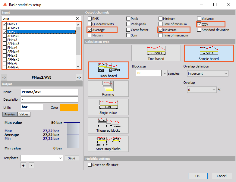
Basic statistics of angle domain data

The example settings on the image 56 are based on cycle-based data: one value per cycle. The basic statistic can also be calculated from angle based data. For example the maximum pressure curve over a defined number of cycles.

For the angle-domain data statistics and the cycle based statistics you can use the same setup. The only difference is that the output channels of the angle based statistics are vector channels. In the left bottom of the screen, you can see different previews according to the data-types. The cycle-based channels show a value and the angle domain-based shows a data curve (of the vector channel).

You can also mix different input channel types in one statistics module: time domain, angle domain, or cycle-based data. The statistics mathematics will always use the correct output channel types for the corresponding input data types.

Array statistics

For analyzing angle domain data the array statistics can be used. Array statistics can be added in the Math module -> Add Math -> add Basic statistics. The screen similar to the one on image 58 should have opened.

This module accepts only input channels as a vector type (angle domain data). The output is always a single value calculated for each vector. So using the array statistics on CEA data, the result is always a cycle based value.

Array mathematics

Another powerful tool for manipulating data from the CEA module is the array mathematics inside the Formula setup. Only array (or vector) data are allowed as input channels. So this mathematics can be used with angle domain data from the CA Module.

This can be added in Math module -> Add Math -> add Formula.

Below a short summary of the functions is described:

With the functions min, max, and avg we have the same functionality as the array statistics. But we have also access to a single data point of an array when using [ ] or { }. 

The formula on the image 58 subtracts the value at -30° of its vector:

1'PCyl2'-'PCyl1'{30}

Or in other words, the additional CA channel is offset compensated with the value of -30°.

It is also possible to cut data of an array:

1'PCyl2'{-30:60}

As a result we will get a new array containing the data from -30° to +60°.

Automatic display mode

When you start the measurement, DewesoftX will automatically generate a display setup (aka. measurement screen), named CEA, showing the major signals for a quick start. The tooth wheel symbol on the CEA display icon indicates that this display is generated.On the image 60, the automatic display configuration is shown. The orange squared visual control is a 2D diagram, which can be assigned to an angle based result channel.

The handling of all visual controls follows the same concept. For the selected visual control the properties are shown on the left side. The channel selector for this visual is shown on the right side. Only channel types suitable for the selected visual are shown. E.g. you can't select statistic channels for a visual control that expects angle based data. The channels that are currently selected are shown in bold.

Customizing displays

DewesoftX allows full customization of the measurement screens: i.e. you can add/remove and rearrange all visual controls to your specific needs. The major visual controls for combustion analyser measurement are described below.

Overview of data types

Not every display can handle every data type. Different input data sources generate different data types. Different mathematic functions generate different data types as well. Moreover, the result of mathematical functions may depend on the input channel type as well.

For example: the CEA module will use the time domain data as input and generate primarily:

• angle domain data aligned to the combustion cycle, and

• cycle-based data which holds one value per cycle.

Let's make a summary of the different data types with some examples of the sources and which visual controls can be used for the different data types.

Scalar (single data points)

Scalar channels contain one single value per timeslot (i.e. in comparison to Vector or array channels, which contain multiple data values per time slot). Depending on how they are acquired (or calculated), we divide these channels into three groups:

• Synchronous,

• Asynchronous, and

• Single value.

The most common channels, are the synchronous channels which are usually analog, counter, or digital input channels as well as simple mathematical operations that depend on these channels.
Synchronous channels are time-domain data with equidistant time between the samples. The time distance is defined by the dynamic sample rate (except for external clocking).

Asynchronous channels are for instance CAN bus or GPS data. But also mathematic functions can result in asynchronous channels. For example:

• the result of block-based mathematics, like the statistics, output

• all cycle-based data from the CEA module (eg. MEPx or MaxPressure)

Single value channels contain only one single value per measurement. For example:

• constants, like header variable

• the output of mathematics like:

  • Overall statistic calculations  from the CEA module

  • basic statistics

For all of these scalar channels various visual controls are available in DewesoftX. Some examples are Digital meters, Recorder, Analog meter, Bar graphs, and so on, ... XY-recorder can also be used to visualize this data.

Vector or array channels

In contrast to the scalar data channel, vector channels (aka. Array channels) contain multiple data-points for each time-slot.

Examples:

• One FFT shot consists of multiple amplitude values - one for each frequency of the FFT resolution.

• Angle-domain pressure is stored as vector data - for each vector we get all pressure values over the defined angle resolution.

2D-Graphs are designed to display these data types. There are some special 2D-graphs dedicated to CEA:

• the Combustion scope

• the PV-Graph

3D-Graph allows you to display a history of these data channels (the time is the third dimension)

Matrix channels

Matrix channels are multidimensional vector channels. For example in a 2-dimensional matrix channel, each time-slot will contain an array and the elements of this array are also arrays (which contain the data in the array elements).

The output of complex sensors like a Thermo-Camera is matrix. This data can be shown in a 3D-Graph.

CEA-scope

The CEA-Scope can be used for all angle based data from the CEA-mathematics. The results can be shown from actual data, from running or overall average, and as well from the additional channels.

Combustion PV-graph

The p-V graph (Pressure over Volume) can show actual and averaged pressure data.

Standard display types

Cycle based results such as MaxPressure are calculated for every cycle. We get a single value every two revolutions for 4 stroke engines, and one value for every revolution in 2 stroke engines.

Cycle based results can be shown in various displays. The common displays for cycle-based results are: Digital, Analogue, Bar, and Recorder.

You have several options to start and stop storing:

• manually, and

• automatically with various settings of the trigger conditions.

Manual start-stop storing

If you want to manually start-stop storing, select the Storing type: always fast. Find the Storing settings on the location: Measure -> Ch. setup -> Storing. You can start storing your data directly in the setup screen by pressing 'Store'. Or you can first go to Measure to first take a look at the live data and then start storing whenever you like.

To stop storing, just press the Stop button.

Pressing Pause will stop storing the data. When you are in pause mode you have 2 options:

• press Resume to continue storing, and

• press Stop to end the measurement and close the data file.

When you stop the measurement, the overall statistic values are stored in the data file. The illustration below points out this difference more clearly. When you look at the graph you can see 2 marked ranges:

• The Stored data time: this is the time from the start of storing (when we have pressed the Store button) and when we have pressed the Pause button).

• The Average calculation time: this is the full time shown in the graph:
  after pressing Pause, the measurement still continues (and the statistics will still be calculated), but the measurement data will not be stored in the data-file. But when we press Stop at the end, the value of the statistics will be written to the data-file.

The overall averaged result (the green channel: Cyl/Ave/P1/MaxP) does not match the expected average of the data values (blue channel: P1MaxP) within the Stored data time range (because the calculation continued after pressing the Stop button).

 When you open the data-file in Analyse mode, the recorder will only contain the data of the Stored data time range and the average value will not match the expected value (average will be calculated from store start to stop).

When reloading this data file it seems now that average calculation is wrong because you can't see anymore the complete data set that was used for the average calculation. To correct this it is possible to recalculate the complete the CEA-mathematics out of the stored data file again.

Press Offline math, enter the CEA module setup, and change the calculation state of the module from Calculated to Offline.

Go back to Review and you can Recalculate the CEA mathematics. The overall averaged pressure channel now matches the stored pressure data. Press Save to overwrite the original stored CEA data inside this data file.

Storing a defined number of cycles

DewesoftX offers various trigger conditions for starting and stopping the acquisition. When you want to store a fixed number of cycles, then you can use the Stop storing after XXX CEA cycles feature. In the example below, storing will be stopped after 100 cycles.

Start-stop on channel condition

The aim of triggered storing is to store on external events. The start and the stop trigger can be any channel. Additionally pre-trigger and post-trigger time can be defined.

Dewesoft X offers various trigger conditions for starting and stopping the acquisition. As described in chapter Manual Start-Stop storing we need to take care of the calculation method of the overall statistics values to get the expected results.

For triggered start and stop storing, you must select the Storing type: fast on trigger. Now we have the possibilities to define Start storing and Stop storing conditions.

Let's make one example when storing should be started if the maximum pressure is above 100 bar and should be stopped after 100 cycles.

Start storing condition type is a simple edge on channel P1/MaxP.

Stop storing condition is channel Cycle count. As Mode we need Delta amplitude to stop after 100 cycles.

This will already work (e.g. it stores only the data of the 100 cycles), but we also need to take care of the overall statistics. With the current settings, the data-file will remain open after the 100 cycles and the overall statistics will remain active.

To avoid this, we can enable Stop storing after 1 trigger: This means that the storing will be stopped after 100 cycles and the DewesoftX data file will be closed (and will contain the overall statistics for the 100 cycles). When the next trigger occurs a completely new data-file will be created.

With the settings above, the average channels are reset at ARM of measurement. So the Average channels will include the cycle value before the trigger event occurs as well. If average values are required for further analysis, they must be recalculated in post-processing like described before.

In the Analysis mode of Dewesoft X you can load a data file and:

• review the data,

• modify or add math modules, and

• print the complete screen to generate a report.

For analyzing recorded cycles the yellow courser can be moved to browse through the cycles.

Similar to the Measurement mode you can modify or add new Visual controls or Displays. All these modifications can be stored to the data file with Save file changes 

You can also load the measurement screen layout and formulas from another data file with Load display and offline math.

By pressing Edit on the right top corner a context menu is opened which gives you the possibility to copy the image or as well the data shown on the actual display to the clipboard or to a file.

If further analysis is needed, various export data formats are supported.

Time-domain data

When opening a Combustion analyzer data-file, the default Export Properties is set to Combustion data. To export in time domain, export properties must be set to Full speed data in the Data presentation option. This means time domain data is exported. Angle based data from the CEA module are exported as a vector (if the target export format supports vectors). They are time-stamped to the end of the cycle time (the same is true for all cycle-based results).

The Channel list gives a quick overview of the channel type (Dimension) and update rate (values per second).

Angle-domain data

To export angle-domain data we have to change the Data presentation to CEA data. With this setting all output channels from the CEA module can be exported as angle-domain data.

The results can be categorized into 4 groups:

• Cycle data as Vector: Angle domain data like pressure, integrated heat-release, additional channels...

• Averaged Cycle data as Vector: One angle vector for the complete measurement like the average pressure.

• Once per Cycle data as Scalar: Cycle based data like max. Pressure (value and position), I50, MEP values...

• Averaged Cycle data as Scalar: One value for the complete measurement like average of max. Pressure.

Before exporting the data we have to define the x-axis base.

The table below gives an overview of the difference in x-scaling using the different export types:

File replay

It is possible to export analog channels into a file that can later be used to simulate analog channels, without having any hardware connected. If we have an analog angle sensor signal recorded, we can export that together with the pressure signal channel(s) and simulate a running engine.

First, the extension for replay file export must be added. This can be found in the download area.

After that, extract the file into: <Dewesoft_installation_path>\Bin\Addons\

The next step is to run Dewesoft as an administrator to register the extension.

We can export any recorded data file, where we stored the analog inputs.

In the file export, we must first select the Data presentation option and choose the Full speed data type. Then we can select Replay (*.rpl) export format. We can use the channel filter to find and export all Analogue (AI) channels. We can export also synchronous mathematics channels, which will act like analog channels in file replay.

CAN interface

The Dewesoft combustion engine analyzer can acquire and transmit CAN messages. When transmitting is used, any measurement result can be sent to any other host system (for example INCA).

1. Add a transmit channel by pressing +Tx button in the CAN tab.

2. You can define the CAN-Identifier (arbitration), its name, and as well as the DLC (Data Length Code).

3. Define the channel types inside the identifier with the Data Format, Data type, Start bit, Length, and the scaling.

4. Now we define a transmit event for this CAN message:

• Periodic: The interval time can be set in milliseconds.

• OnButton: A control button in the Measurement Mode can be assigned to this event.

• OnStart: When changing to the Measurement Mode with definable delay in msec.

• OnStop: When the measurement is stopped.

• OnTrigger: A measurement channel condition defines when the data should be sent.

• BeforeMessage: You can select another message and this message will be sent before that message.

• AfterMessage: You can select another message and this message will be sent after that message.

5. Select the data to be transmitted: Constant values or any measurement channel can be selected

6. All the defined transmit channels can be exported to a DBC-file for later import on the Host system.

The average delay time for CAN Out data will be around 100 msec because the complete cycle is acquired first and after the calculation the data is available for the output.

Testbed

The communication to the testbed server is implemented as a dedicated Plug-In. You can choose between:

• AK Protocol,

• Puma Open AK,

• D2T AK, and

• Tornado AK.

For all of these protocols the RS232 or TCP/IP connection is possible.

Detailed information about the plugin usage and setup is available in the combustion engine analyzer manual, chapter 9.

In Dewesoft we can use the file replay option to simulate analog input channels and create a CA setup and also test the functionality of CA.

First, the extension for replay file export must be added. This can be found in the download area.

After that, extract the file into: <Dewesoft_installation_path>\Bin\Addons\

The next step is to run Dewesoft as an administrator to register the extension. When Dewesoft starts, open Settings to configure file replay and switch Dewesoft X operation in Offline mode. Then click on the Simulated devices and set the Simulated channels mode to File replay. See the image 85.

Exported *.rpl file can be used or you can download a test file. When the file is selected there will be information on how many channels are simulated, what was the sample rate and the total length of the file. The replay file is always in the time domain. Select also the option repeat, to loop the file, otherwise it will be played only once. Only analog synchronous channels will be replayed.  

After that, close settings and create a new setup.

If we go to channel setup we see that we have 9 simulated analog channels. We need to find out what these channels are and we can do this by simply enabling all channels and going to measure.

On the recorder display we can see all 9 channels at once and can also freeze the data and zoom in to one part of the data. From this we can quickly see that the first channel is the angle sensor and the other 8 channels are pressure signals. The angle sensor in this case is a 60-2 sensor.

We can rename the channels for easier setup, select physical quantities, and set the scaling. We will create a 4 cylinder CEA setup. 

Now we need to add the CEA module.

In the Engine settings of the CEA module we first define the cylinder count, enter the geometrical data of the engine, fuel type, select the appropriate pressure signal for each cylinder and input the ignition misalignment. After we have entered all the information we can save then engine as a new template. The only thing we need to do next is to define the angle sensor setup.

In the next tab of the CEA setup, we select the type of angle sensor as a 60-2 and also the channel this is connected to. We should immediately see something on the p-V preview diagram (left) and also the pressure signal in the angle domain (right). If the angle sensor was defined correctly we should see stable and correct RPM on output on the right and also 60 pulses per revolution.

We can see that the peak pressure on cylinder 1 is around 100degCA. This means that we have an offset of the angle sensor. If we would have a replay file from a non-fire engine, we could do TDC detection, but since this a file with combustion, we have to enter the offset manually. In this case we know that the offset is 80deg.

When the trigger offset is correct, we can see that the pressure curve is shifted to the correct position, and also the p-V diagram shows a correct output.

If we switch to the Result definition tab we can also immediately see the rate of heat release output and accumulated heat release.

Now we can go to measure, and on the predefined CEA measure screen, we will already have all the basic combustion analysis information as it is shown on image 93.

CEA can also be used in combination with other modules. When using it for a 4-stroke engine, we get a possibility to review data in the angle domain for a complete engine cycle - 720deg.

This can be very useful to analyze vibration data for a 4-stroke engine, otherwise, we see the data only in a 360deg cycle, as shown in the image 94.

The following is just one example of how CA can be used for other purposes or to convert time-domain data into angle domain data. We only need one angle sensor which is valid for CA and one input. The input can be any type - either some analog input or math channel or even an output channel from some other module (torsional vibration, power analysis, order tracking, modal test,...).

Torsional vibration & combustion engine aalysis

Please refer to the ProTraining for detailed explanation about the Rotational and torsional vibration module.

To use the vibration analysis module together with CAA, only one angle sensor is needed. First we add the Torsional vibration module.

Sensor input and sensor type must be selected. The rotational angle must also be selected for output.

If there is another sensor mounted on the other side of the engine shaft, then we can select also the other sensor and activate the output calculation for the torsional vibration angle.

We must also add the CEA module and configure the angle sensor input.

For the Encoder settings we only need to select a pressure sensor - in this case, Encoder-1024 and the counter location to which the encoder is connected to.

Under additional channels in Engine settings, select the output from the torsional vibration module. All additional channels will be shown in the angle domain. If we also have an encoder on the other side of the shaft, and have torsional vibration results, we can also add additional channels. We can select all three outputs for conversion into the angle domain. See the image 98.

When we go into the Measure mode and enable the Design mode, we have two additional display types available from CAA. We add a Combustion scope to display the data in the angle domain for a complete engine cycle.

We can display all three vibration channels at once on the graph. Pressure or other channels can also be added.