Basic Measurement with Dewesoft DAQ Hardware

Course overview

This course is an introductory hands-on tutorial designed to guide new users through their first measurement with Dewesoft tools. It begins with installing DewesoftX, which is freely included with DAQ devices and usable for analysis even without a license.

Once the SIRIUS DAQ unit is connected via USB, users will experience DewesoftX’s intuitive auto-detection of device serial numbers, power connectivity, and sync status. The session then transitions into hardware setup:

• activating analog input channels,

• selecting input modes (e.g., IEPE for accelerometers),

• picking dynamic acquisition rates (default ~20 kHz), and

• leveraging TEDS support for automatic sensor configuration and calibration warnings.

Participants proceed to perform live measurements using accelerometers, tuning forks, strain gages, and encoders. They’ll capture dynamic events using the recorder display and learn basic workflow in both Measure (live data capture) and Analyse (post-processing) modes—zooming into events, selecting sections via cursors, and preparing data for export.

The course concludes with exporting recorded data in multiple formats—Excel, CSV, FlexPro, UNV—and demonstrates how to export only selected time regions. Additionally, you’re introduced to Dewesoft’s simple math module for baseline signal analysis and learn how to use various data storing modes, including fast-on-trigger features and naming conventions, to streamline measurement sessions.

By the end of this course, you’ll be confident in your ability to set up and perform basic measurements with Dewesoft hardware, process the data, and export it for further analysis or reporting. Perfect for those starting with DAQ systems in fields like vibration, encoder-based motion tracking, or strain measurements.

First, you need to install DewesoftX on your computer. Download the DewesoftX software from our [download page], then run the installer. DewesoftX supports Windows operating systems, version 7 (32-bit and 64-bit) and newer.

Licensing

• The license for measuring with DewesoftX is included in the device (usually the PROF version). Once the device is connected to the USB port, it acts as a dongle.

  The license for analysis is free! DewesoftX can be installed on any computer, and stored data files can be opened, recalculated, and exported without additional cost.

  Additional licenses may be required for plugins, which can also be written into the Dewesoft® device. To test plugins, you can request a 30-day Evaluation License.

In this simple measurement lesson, we will demonstrate basic measurements of various sensors using the Dewesoft SIRIUS system. Each sensor will be connected one after another, and a basic measurement will be performed. It makes sense to follow this process from start to finish, as each measurement introduces more details, different instruments, and additional functions. In the picture below, you can see the demo equipment that was used.

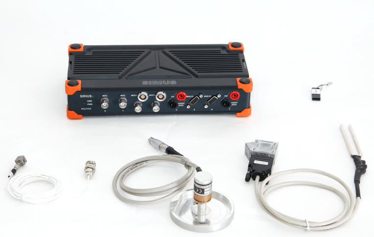
The demo kit consists of the SIRIUS device, its installation USB stick, and three sensors:

• Acceleration sensor

• Tuning fork

• Encoder

Dewesoft X launcher

When the power and USB connectors are connected to the computer, DewesoftX will automatically open from the auto-detect screen and display the devices with their serial numbers, the power supply status, and the status of the synchronization cables if more than one unit is connected. Pressing Run Dewesoft will close the pop-up and start the DewesoftX software.

Manual setup of hardware

If you need to manually set up the hardware, start DewesoftX and go to Options → Settings.

Under Devices, set the Operation Mode to Real Measurement. Then scan for the hardware using the Refresh button. The SIRIUS device will be detected according to its serial number.

When you confirm the settings, the Channel Setup screen will appear in Measure mode, showing the instrument with its built-in amplifiers.

Notice the two buttons in the upper-left corner: Measure and Analyse. The Measure mode is used for storing data, while the Analyse mode is used for reloading and analyzing data files.

We connect an IEPE accelerometer to the first channel.

First, consider the required sampling rate. What is the highest input frequency you expect? In the Dynamic Acquisition Rate drop-down menu, the default value is usually 20 kS/s, which is sufficient for now.

If it is not already set, activate the channel by setting it to Used.

Since the SIRIUS-ACC amplifier supports two input modes, set the Measurement field from Voltage to IEPE in the row of the first amplifier. This ensures that the amplifier supplies the sensor. If the Ampl. Name (and the LED ring around the BNC connector on the instrument) turns green after a few seconds, the sensor impedance is confirmed as OK.

Finally, open the Channel Setup window by pressing the Setup button.

Channel setup

The Channel Setup window is divided into two sections: the left side (Amplifier Settings) and the right side (Sensor Settings). You can also change the channel name here.

Amplifier Settings – With the Dual Core option enabled (if you have a Dual-Core SIRIUS), there is no need to adjust the input range. At the bottom, you can see a quick preview of the sensor signal—tap on the accelerometer to test it.

Sensor Settings – In our case, the accelerometer has built-in TEDS (Transducer Electronic Data Sheet), so all calibration factors and calibration data (though in this case out of date, as indicated by the red warning) are read automatically. Otherwise, you must manually enter the physical quantity (Acceleration), the unit (g or m/s²), and the calibration factor. Alternatively, place the sensor on a reference shaker and press the Calibrate button.

Storing

Before starting the measurement, go to the Storing ribbon and specify a file name. The storing type is set to Always Fast by default, but you can define trigger conditions later if needed.

Then click the red Store button to begin recording the measurement.

Recorder

DewesoftX switches to Measure mode. For faster navigation, there are two screens at the top: Recorder and Custom (predefined). These screens contain instruments and can be freely customized. The Recorder screen currently consists of one Recorder instrument.

Tap the accelerometer a few times.

The Recorder y-axis automatically adapts to the currently visible minimum and maximum values if the Autoscale option in the Recorder properties (on the left) is enabled. On the right side is the channel list, showing the channel currently assigned to the Recorder instrument.

After completing the measurement, click Stop, then switch to Analysis mode.

Analysis

Let’s take a look at the recorded data. You are now in Analysis mode. The last recorded data file is automatically reloaded. Let’s zoom into one of the peaks.

To zoom in, press and hold the left mouse button while moving to the right, then release it. If you move the mouse between the two cursors, a small + sign appears next to the mouse pointer. Clicking between the cursors will zoom into the selected area.

To zoom out to the previous level, simply right-click.

You can zoom in until the sampling points (20 kHz) become visible.

Export

Only the selected region (shown in the overview instrument at the top) will be exported.

Go to Export → File Export, choose the file type and properties, enable or disable channels on the right, and then click the Export button.

The FlexPro and MS Excel ActiveX ribbons at the top allow you to export directly into a template, which you can adapt for inclusion in your finished report.

We connect a strain gauge to one of the STG inputs of our SIRIUS device.

A tuning fork is normally used for tuning the instruments of an orchestra. It is tuned to 440 Hz, which is the standard pitch for the note A. In our demo tool, a quarter-bridge strain gauge with either 120 Ω or 350 Ω resistance (marked on the connector) is mounted on the steel. This allows us to measure the strain caused by the vibrations.

Open the setup of the channel to which the tuning fork is connected.

In the upper-left section, you will find the amplifier settings. Set the mode to Bridge and Quarter Bridge 3-wire, with either 120 Ω or 350 Ω (marked on the connector). The corresponding circuitry is shown, illustrating how to connect the quarter bridge to the 9-pin DSUB connector.

Select an appropriate range. If you use the highest range, you do not need to worry about overload (input voltage exceeding the amplifier range). In this example, we use a smaller range, e.g., 20 mV/V. The higher ADC is now operating in the 20 mV/V input range, while the lower ADC input range is 5% of that (1 mV/V) simultaneously, providing excellent dynamic performance.

On the right side (Sensor Settings), select the physical quantity (Strain or Stress) and the appropriate unit. If your sensor includes a TEDS chip, all the settings will be read automatically.

Balance sensor

Before starting the measurement, the strain gauge must be balanced. Click Balance; the output will reset to 0 µm/m, and the offset will be displayed next to the button.

Sampling rate

Since the natural frequency of the tuning fork is 440 Hz, we need to consider which sample rate to use for digitizing the signal. In theory, a factor of 2 (880 Hz, according to the Nyquist criterion) would be sufficient. In practice, however, it strongly depends on the signal characteristics. We recommend using a factor of 10 or even 20 to achieve reliable results.

Therefore, a sample rate of 20 kHz is still appropriate.

Go to Storing, specify a file name (e.g., tuning_fork_measurement), and then click Store.

Scope widget

Next, switch to the Custom display and add the Scope widget. Maximize it to fill the entire screen.

Switch to the Scope screen. Strike the tuning fork to generate an oscillating signal, then click the y-axis label to apply min/max scaling.

Set the Trigger to Auto in the properties panel on the left. Move the trigger level up or down with the mouse until a stable triggered image appears.

Use the +/- buttons on the x-axis to adjust the displayed time window.

Customizing displays

Next, add an FFT instrument to measure the resonance frequency of the tuning fork. The Custom screens are usually empty, allowing you to add any widgets you like. Regardless of which display you use, every display can be adapted to your needs.

Design mode

Enter Design Mode either by clicking the Design tab at the top or by starting to add widgets via the Widgets tab.

In the Widget Search window, type FFT and add an FFT widget to the display.

By default, the channel AI 5 is automatically assigned to the instrument, as it is the only channel currently set to Used.

While in Design Mode, you can freely resize the FFT widget and move it to your preferred location on the screen. Once the FFT diagram is adjusted to your needs, exit Design Mode by clicking the Design button.

FFT instrument

The following steps will help you display your data quickly using the FFT:

• Y Scale Type: Set to Log.

• Y-Axis: Adjust according to the measurement range. In this case, it is set from 0.001 to 1000 µm/m.

• Measured Peak: Click on the peak when the tuning fork is vibrating. The peak values will be displayed, showing a maximum of 439.5 Hz with the corresponding amplitude.

Analysis folder view

After stopping the measurement, click the Analysis button and go to the Data Files tab. The Analysis folder view will appear, which functions like Windows Explorer. At the bottom, you will see information about the channels and data header. Using the powerful search fields, you can easily find the data file you are looking for.

Now connect the demo encoder to, for example, ACC+, STG+ (with an additional Lemo connector), or the MULTI module.

By default, the Counter inputs are not visible in DewesoftX. You need to add them using the + More button.

Additional software options can also be added here, for example, Power, Order Tracking, or Modal Test. The Counters will then appear as a ribbon at the top.

The buttons on the top can be customized. Click the + button again, go to New Setup Defaults, and select the asterisk for the Counters. From now on, they will appear by default each time you start DewesoftX.

There are two typical counter techniques:

• Gated measurement (typical for high-frequency ranges > 100 Hz).

• Pulse width measurement (typical for low-frequency ranges < 100 Hz).

Many applications require both counter information and analog data. Traditional systems do not provide counter information synchronized with the A/D converters, because they receive the counter data only after the gate time or after the measured pulse time.

In contrast, DewesoftX real-time counting uses an additional counter with a 102 MHz time base to determine the exact time of the signal’s rising edge. This unique feature enables the calculation of the exact counter value at the A/D sample point (e.g., value 1.87 in image 24), compared to standard counting with software interpolation (e.g., value 1.5 in image 24).

When you turn on the encoder, the Counter value should begin increasing. Each counter (CNT x) consists of three digital inputs (IN0, IN1, and IN2). Set the channels to Used and open the Setup.

Counter setup

In our case, we are using a 1024-pulse encoder with A, B, and Z tracks. Set the basic application to Sensor (Encoder) and the sensor type to Encoder-1024. Enable Encoder Zero so the angle resets with the Z pulse once per revolution, and also enable Automatic Angle Wrap Around.

The most important output channels are Angle, Frequency, and Raw_Count.

Go to Design Mode and add an Analog Meter, Digital Meter, and Recorder. Set the properties for each instrument on the left (minimum value, maximum value, and resolution). To assign or unassign a channel to an instrument, first click the instrument, then select or deselect the channel from the channel list on the right.

Analog and digital meter

Below are some example properties for the analog and digital meters. These should help you display your RPM signal.

Save the setup

After completing all sensor settings and creating your custom screen, you can save the setup/display configuration as a setup file (*.dxs). To do this, stop the measurement or return to Channel Setup, then click the DewesoftX icon button and select Save Setup As...

In the same way, you can load any configuration.

In DewesoftX, there is an extended math library along with several software modules for special applications. Let’s look at one of them as an example—you will find many more. In this case, we will use the Power module to calculate active power and measure grid frequency.

First, add the Power Analysis module using the + More button.

There are several settings and calculation options, but for a basic measurement, we only need to assign the correct channels. For U1, select the voltage channel, and for I1, select the current channel.

Go to the Measure screen, where several predefined displays related to the Power module will be shown. You can also create your own display, combining power with other parameters.

After setting the input and math channels, we are ready to perform a measurement. Store some data by pressing the Store button. Once the data is stored, press Stop to end the recording.

By pressing Analyse, the file can be opened for analysis. You can view different screens, and by pressing Play, replay the recorded data.

For data analysis, DewesoftX offers several possibilities. You can perform Offline Math inside the software, export data to other software packages, or simply print the display you would like to include in a report. All standard file operations, such as merging files, renaming them, or deleting them, are also supported.

By selecting the Print button, the chosen display will be printed.

You can also export data in various formats (Excel, MATLAB, DIAdem, FlexPro, …) by selecting the Export function.

If you want to perform additional analysis on already stored data, you can easily use Offline Math inside DewesoftX. In this example, we will calculate vibration velocity from an acceleration signal. To do this, select the Offline Math button.

Click the + Add Math button and, in our case, select Time Integration/Derivation.

In the setup, select the acceleration channel on which integration will be performed. Note that the system will automatically suggest the unit of measurement as mm/s and apply the conversion. You can, of course, choose an alternative unit, such as ips.

After completing this step, go back to Review and add a Recorder display. Place both the acceleration signal and the calculated math signal (vibration velocity) on it. To calculate the math signal, click the Recalculate button. You will now see both signals displayed.

There are many things you can do in DewesoftX, and we invite you to explore further sessions on different topics, such as How to Measure Signals, How to Analyze Data, and How to Use DewesoftX.

Sine wave on all channels

If you set the Operation Mode in DewesoftX to Simulation, you will see a display similar to the one below—sine waves with random amplitudes and frequencies on all channels.

When you switch back to Ch. Setup, the amplifiers will display Demo-.... In this case, please refer to the section above titled Manual Setup of Hardware.