

What You’ll Learn 📍
Understand the Virtual 3D Polygon environment and its use in GNSS and vehicle dynamics testing
Install and enable the Polygon plugin (plus optional Vehicle Simulation) in DewesoftX
Set up Global or Dynamic Origins using GNSS coordinates for accurate real-world alignment
Define and manage Objects—static or moving—with position (GPS or offsets), geometry (points, lines, polygons), and 3D models for visualization
Conduct Geometric calculations: distance, timing offsets, group-based metrics, and Time-to-Collision (TTC) between objects
Visualize and animate setups in 3D using Dewesoft’s Map widget and Polygon preview pane, both live and offline
Apply Freeze/Unfreeze logic for multi-run tests, brake tests, lane departure scenarios, and more
Analyze recordings in DewesoftX using synchronized GNSS data, 3D object motion, and virtual environment scenes
Course overview
The course teaches you how to create and use a virtual testing environment—Polygon—within DewesoftX. Originally designed for vehicle dynamics and ADAS (Advanced Driver Assistance Systems) testing, Polygon enables accurate alignment of real-world GNSS data onto a virtual 3D map plane—useful in automotive, marine, heavy machinery, and robotic applications.
You’ll start by installing the Polygon plugin (Polygon.dll) and optionally the Vehicle Simulation plugin to generate test trajectories via keyboard or joystick input. You’ll then set up an origin in global GNSS coordinates or dynamic mode to ensure precise alignment. Adding objects—using GNSS data, static positions, or relative offsets—you’ll define geometry and visualization features like 3D models and bitmaps.
Next, the course dives into performing calculations: measure real-time and post-acquisition distances, timings, TTC between moving/static objects, and group-based metrics. You’ll see how to freeze object states to capture events like tire stop points or lane encroachments, enabling brake test and lane-departure analysis. The Polygon preview pane and Map widget allow reviewing movement and object interactions in 3D, with visual synchronization to GNSS data channels.
By the end, you’ll understand how to integrate Virtual 3D Polygon into your workflow—setting precise GNSS origins, configuring objects, running simulations or live tests, and interpreting spatial data in a customizable virtual space. This empowers you to conduct advanced positioning analyses, trajectory visualization, and spatial validation for dynamic systems with DewesoftX.
Introduction to the polygon
Polygon is a platform designed for tests involving moving objects. It was developed specifically for vehicle dynamics testing and advanced driver assistance systems (ADAS), which help improve traffic safety. Polygon provides a visual representation of measurements in a three-dimensional virtual space and offers easy-to-use tools for geometric measurements between multiple static or moving objects. Visualizations and outputs can be generated either during measurements or later in offline mode.
Thanks to its flexibility, Polygon is not only used in the automotive industry but also in marine applications, heavy machinery, and more.


How to install the polygon plugin?
Polygon is a platform designed for tests involving moving objects. It was developed specifically for vehicle dynamics testing and advanced driver assistance systems (ADAS), which help improve traffic safety. Polygon provides a visual representation of measurements in a three-dimensional virtual space and offers easy-to-use tools for geometric measurements between multiple static or moving objects. Visualizations and outputs can be generated either during measurements or later in offline mode.
Thanks to its flexibility, Polygon is not only used in the automotive industry but also in marine applications, heavy machinery, and more.


Optional plugin: vehicle simulation
If you want to test Polygon setups before use or learn how to use the Polygon plugin offline, an additional Vehicle Simulation plugin is available — the VehicleSimulation.dll library. The installation process is the same as for the Polygon plugin.
The Vehicle Simulation plugin automatically generates longitude, latitude, and heading channels, which can be used to move vehicles within the Polygon environment. These channels can be controlled using either the keyboard arrow keys or a joystick.

How to setup the polygon?
In Channel Setup, click the Polygon button in the main toolbar. The Polygon setup is divided into two panels. The left panel is the setup panel, where Objects, Origin, and Calculations are defined, while the right panel is the visualization window, which displays a preview of the setup.
To view the Polygon on the measurement screen, place a Map widget on the screen, switch it to 3D mode, and add all the objects. The Polygon display should already be visible by default. Keep in mind that calculations can only be performed between 2D objects.


Objects in polygon
Objects in Polygon are used for both calculations and positioning. Each object is defined by its position and geometry. The position can be measured, predefined, or set relative to another object. The geometry of an object can be defined using multiple primitive shapes such as points, lines, polygons, and arcs.
With a defined position, Polygon can perform calculations between the geometries of different objects or within the same object. Objects can also be visualized using a model. They are managed with the buttons shown in the figure below — you can add (+), delete (-), or move them up and down.


Object list has 5 columns:
Ord.: shows order of the objects (managed with up and down arrows)
C: option to change colour
Name: to edit the name of an object
Display: buttons, to select displayed properties of the object (orange means, that property is visible)
Focus on: with a click, the object is shown from the top in the middle of the preview window
Objects: position
Positon


GLOBAL POSITION of an object can be defined in several ways:
Static Origin – used for static objects with a known position on the test track.
Constant Position – used for static objects with a known GNSS position (latitude, longitude, and heading).
GNSS Channels – used for measured GNSS positions with latitude, longitude, and heading channels.
Navigation Channel – used for measured positions from a navigation channel.
Other Object – used for objects that are offset from another object with a known geodetic position (applicable to all except Static Origin).


With Offset from Global, you can shift the local coordinate system of an object. X, Y, and Yaw represent relative positions with respect to the object’s global coordinate system. The relative offset can be defined using either a static value — in meters for X and Y offsets and in degrees for the Yaw offset — or by assigning a channel (X/Y/Yaw channel). The offset is applied in strict order: first the translation, then the rotation.
Velocity channels are required only for Time to Collision (TTC) calculations. Channels used for TTC calculations must provide velocity in m/s. Time to Collision is defined as the time before a collision occurs between vehicles, objects, or subjects if their speeds remain unchanged and their paths are maintained. If no velocity channel is defined, a value of zero is assumed, which can also be explicitly specified. The formula for Time to Collision is:
Objects have an additional “Freeze Position” option. If it is set to Freeze or Freeze–Unfreeze, additional channels must be assigned to define when the object should freeze (Freeze input) and when it should unfreeze. You can choose between Positive and Negative crossing, as well as specify the Level at which the object freezes.
If only Freeze is selected, the object will remain frozen until the end of recording. Otherwise, the Unfreeze input must be used to release the object. The Freeze–Unfreeze function is especially useful for performing multiple consecutive brake tests within a single data file.
Objects: geometry


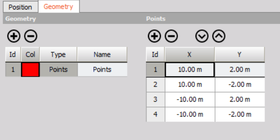
Points
Points are added with X and Y coordinates. In one geometry of points, there can be multiple points added.

Polyline

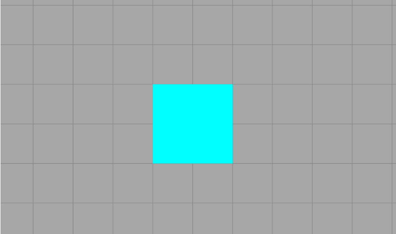
Rectangle
Choose the X and Y coordinates to define the position of the rectangle’s center. You should also define the rectangle’s size by specifying its length and width.

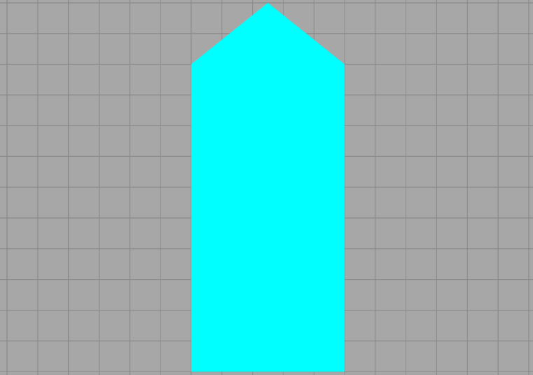
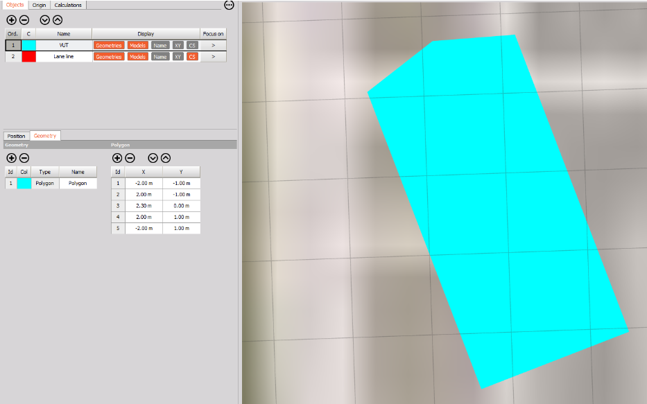
Polygon
A polygon is defined by multiple points (X and Y coordinates) that are connected. The local coordinate system of the polygon is located at the point (0,0).

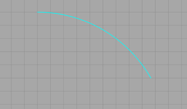
Arc
An arc is defined by the X and Y coordinates of its center, along with the starting angle, sweep angle, and radius.

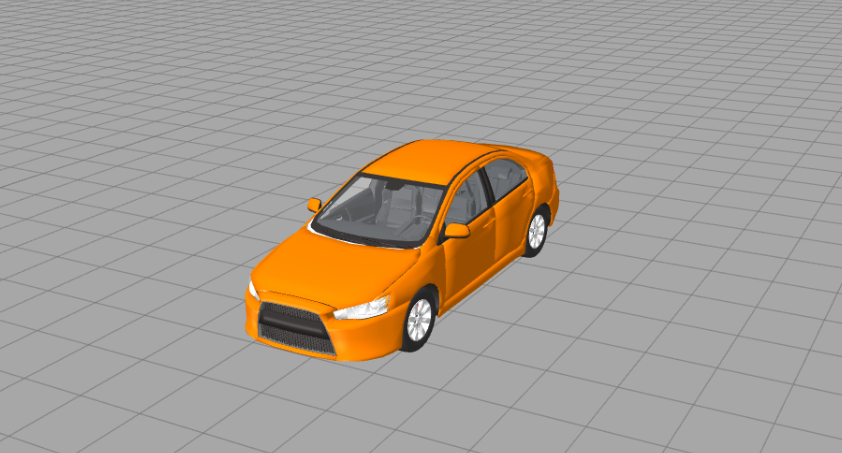
3D model
A 3D model can be added for visualization purposes only. It does not affect the calculations. You can also import your own 3D model into the Map.

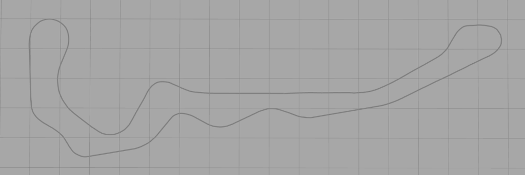
Route
A route is a predefined path (e.g., a track or road) that can be composed of lines and curves. When defining it manually, four elements can be used: Straight, Straight To, Curve, and Curve To. Routes can also be imported. To do this, record a Dewesoft file while driving the route, export it as a GoogleEarth.kml file, and then import it into Polygon. After importing, you can manually adjust the route if needed. If no origin is set, the route import will automatically set the origin to the route’s starting point and align the direction accordingly. The route does not affect calculations.

Origin
Origin
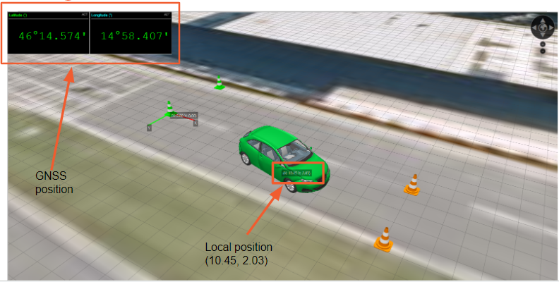
The origin defines the zero point and orientation of the coordinate system on the local plane. All X and Y positions of objects are relative to the origin. There are two ways to define the origin: dynamic or static.
If you choose dynamic, the origin moves with the measured object (useful for vehicle-to-vehicle testing). If you choose static, there are two additional options, described below. When the static origin is selected, offset values for X, Y, and Yaw are available. The main purpose of these offsets is to make fine adjustments during analysis to correct minor inaccuracies.

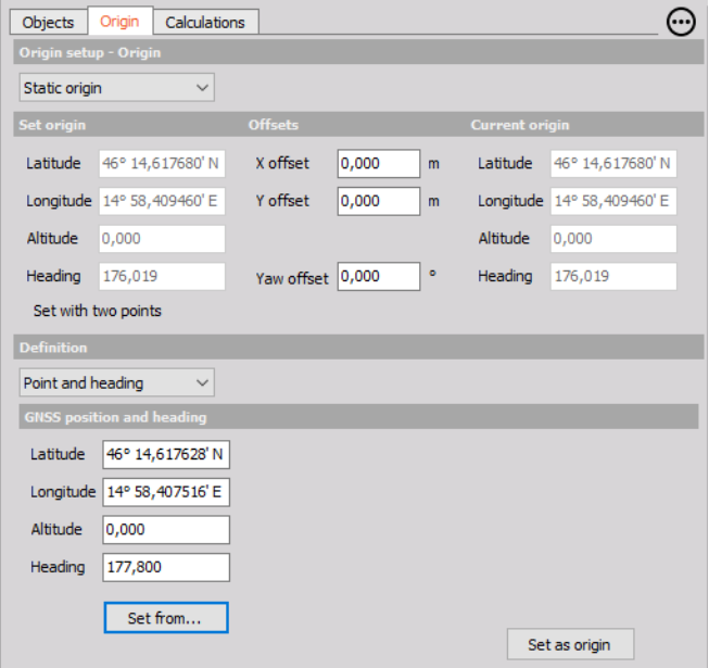
ORIGIN WITH POSITION AND HEADING
Defining the static origin with a point and heading is quick and simple, but not very precise. It relies only on the position and heading of the selected object (entered manually or set using the Setup from… button with the object’s current position). This method can, for example, be used to place virtual tracks on a proving ground, where small deviations are not critical.

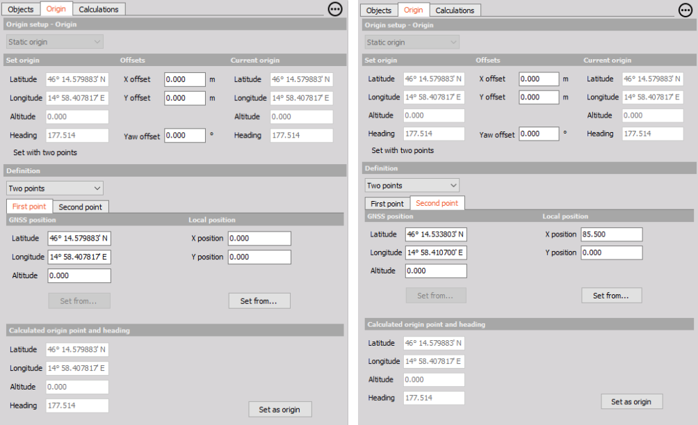
ORIGIN WITH TWO POINTS
Defining the origin with two points is slightly more complex, but it is used when objects fixed on the track (such as cones, points, or lanes) are important for calculations. When setting the origin with two points, ensure that the distance between Point 1 and Point 2 is as large as possible.
To define the points, you must enter both the GNSS position and the local position. The GNSS position can be entered manually or set using the Set from… button, which opens a list of objects that can define a GNSS position. The local position of the points is important because it determines where the measured points are located in real life, allowing them to be transformed into the virtual world’s origin. In this setup, the origin is based on Point 1, while the axis orientation is defined by Point 2.
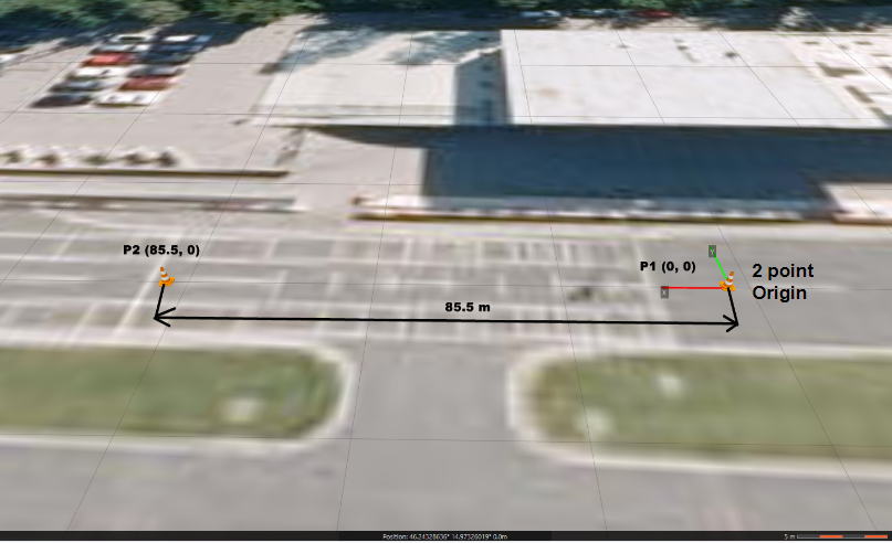
For example, if two points are placed on the same straight line, separated by 85.5 m, the origin will be set at the first point, with the X-axis oriented directly toward the second point.


What the accurate origin is important for?
The origin must be defined accurately to ensure that object positions in the Polygon environment correspond to their positions on the real-world test track. Two common mistakes can occur during origin setup: an incorrect definition of the origin zero point or an incorrect definition of the origin orientation.
An incorrect definition of the origin zero point occurs when the GNSS antenna is positioned incorrectly on the test track and does not match the position defined in the modeled environment. Errors caused by this mistake remain constant throughout the test area, resulting in a fixed offset between the real test site and the modeled objects in Polygon. These errors can be identified by comparing the GNSS antenna’s actual position on the test track with its position (and the connected object) in the Polygon environment.
An error in origin orientation occurs when the GNSS heading is not aligned with the X-axis orientation of the real test site (e.g., when the origin is set using the current position and heading) or when there is a positioning error in the two-point definition. Positional errors increase with distance from the origin; even small orientation errors can cause significant positional deviations far from the origin. Therefore, it is recommended to use a two-point origin definition when high positional accuracy is required in the test area (e.g., for slalom, lane change, or pass-by noise tests).
| Heading angle error | 100 m | 200 m | 300 m | 500 m | 800 m | 1000 m |
|---|---|---|---|---|---|---|
| 0,1° | 0,17 | 0,34 | 0,51 | 0,85 | 1,36 | 1,70 |
| 0,2° | 0,35 | 0,70 | 1,05 | 1,75 | 2,80 | 3,50 |
| 0,5° | 0,87 | 1,74 | 2,61 | 4,35 | 6,96 | 8,70 |
| 1° | 1,75 | 3,50 | 5,25 | 8,75 | 14,00 | 17,50 |
Calculations: setup
In the ‘Calculations’ tab, there are three additional sections: Setup, Groups, and Channels.


Setup
In the Setup tab, the user selects which calculations will be performed and between which groups. There are no default outputs; however, a table is provided where they can be defined. A set of buttons above the table allows adding, moving, or deleting outputs. Each output generates a single data channel, for which both the color and name can be specified. For Distance X, Y and Time to Collision X, Y, an additional channel is also created for alignment. Units are assigned automatically (meters and seconds).


Absolute distance (D) represents the shortest distance between two groups. All types of objects are supported for distance calculation, provided they have defined geometry. The absolute distance is always positive.
Overlap (OL) determines whether two groups of objects overlap. The result can be either 0 (No Overlap) or 1 (Overlap).
Time from overlap (TFO) measures the time between two overlaps within the same group. Multiple objects can be included in a single group.
Time to collision X and Y (TTC) indicates the time before a collision occurs between the involved vehicles, objects, or subjects, assuming their speeds remain constant and their paths are taken into account (in the X and Y directions).
Distance X and Y (DX, DY) calculates the distance along the X and Y axes. These distances can be either positive or negative. The results are always expressed in the coordinate system of the “From group.”
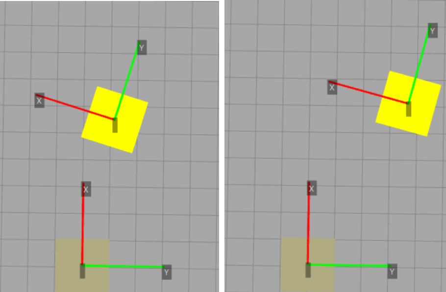
Another output of this calculation is alignment (AX, AY). Two groups are considered aligned if the group being measured lies within the “corridor” of the reference group. The corridor width used for alignment calculation corresponds to the largest dimension perpendicular to the X or Y axis. See the included illustrations: in the first, the objects are aligned; in the second, they are not.

Calculations: groups


Groups are used for calculations. When the dropdown menu is displayed during a calculation, you can select a group. At the top of the tab, there are + and – buttons for adding or deleting groups.
Within a group, you can select one or multiple geometries from the same or different objects to be used in calculations. This is useful, for example, when testing collisions involving multiple objects.
Groups can also be renamed, except for those generated automatically from objects. Automatically generated groups cannot be renamed, deleted, or edited.
Note that visualization objects are not displayed here, since calculations are not supported between them.
For example, if you have several different objects and want to calculate the time from overlap between them, you simply place them in the same group and then include that group in the calculation.
Calculations: channels
Channels

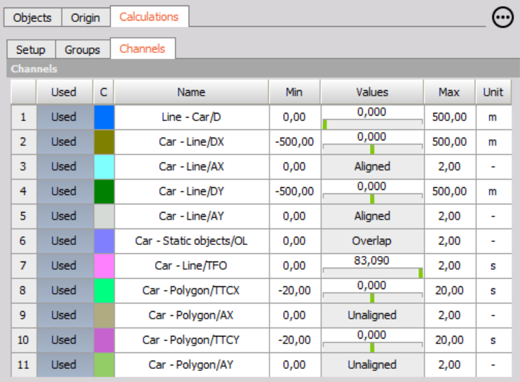
The Channels tab displays all outputs generated from the setup, along with a preview. Channels can be renamed, their colors adjusted, minimum and maximum values modified, and units edited. Channels intended for use on the Measure screen must be switched to “Used.”
By default, channel names are constructed from the names of the groups used in the calculation. The first part is the “From group,” followed by a slash ( / ) and then:
D: Absolute distance calculation
DX/DY: Distance X/Y calculation
AX/AY: Alignment X/Y calculation
OL: Overlap calculation
TFO: Time from overlap calculation
TTCX/TTCY: Time to collision X/Y calculation
How to 3D visualize everything?
Visual settings in the Measure module do not affect the measurement.
Camera mode
Standard view allows the viewing angle to be adjusted manually. The scene can be rotated using the left (or middle) mouse button and zoomed in or out with the mouse wheel.
First-person view cannot be manipulated in any direction; it simulates being behind the steering wheel.
Third-person view can also be adjusted with the mouse (move up or down and zoom). In this mode, the view follows the car and rotates with it. By default, the camera is positioned behind the car, similar to driving simulation games. This view is suitable for driving assistance when following virtual routes.
In the Object dropdown menu, you can select which object to follow.
Layers and models
Since the Polygon works with the 3D map widget, layers can be added. You can create these layers using your own images.


You can also import your own models, which will then be available in the Polygon setup.
Example I: brake test
The Polygon can be used to measure lateral deviations during braking as well as braking distance.
The objects used for these calculations are the vehicle under test, the start of braking line, and the middle line. The start of braking line and the longitudinal line both have Freeze–Unfreeze positions defined, with the velocity channel as the trigger. This means measurement is performed whenever the vehicle’s velocity drops below 49.9 km/h and resumes when the velocity rises above 5 km/h. With this feature, multiple consecutive brake tests can be carried out.
The origin is set to Dynamic Origin because static references on the track are not relevant for these measurements.


Example II: lane departure
Example II - Lane departure
In this chapter, you will learn how to create a basic setup to monitor the distance between the lane line and the VUT. We will use a vehicle simulation plugin, layers from the Vransko proving ground, and the Rimac Nevera model, all of which are available for download here.
For this task, using Polygon, you will learn how to perform a simple Line Assist Warning Test. The origin will be set up with two points that are 85.5 m apart in the X direction:
P1 46° 14.579883' N 14° 58.407817' E (0, 0)
P2 46° 14.533803' N 14° 58.410700' E (85.5, 0)
Now, a straight line should be added to represent the center line of the track. Because the real line has a certain width, the most convenient way to recreate it in a virtual environment is by using a rectangle with a defined width of 0.15 m and a length of 120 m.
Next, add an object with vehicle geometry and assign it a navigation channel from the vehicle simulation. In the vehicle simulation plugin, enter the following coordinates:
46° 14.579883' N, 14° 58.407817' E, Heading – 357.
The vehicle will now be positioned at the Vransko proving ground.

Add the appropriate calculation to measure the shortest distance between the vehicle and this line.
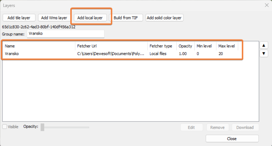
When you enter measure mode and open the Polygon display, you have the option to add layers.

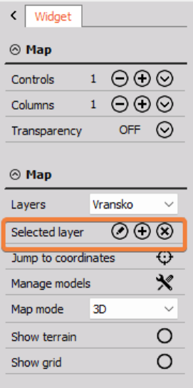
Press the Edit button, and then add a local layer from the Vransko folder, which you downloaded at the start of this task.

After uploading the layers, you also need to load a model. Dewesoft supports many different model formats (.amf, .glb, .gltf, .obj, .stl, .stp, etc.), but we recommend using .obj or .gltf. On the link, you also downloaded Nevera.obj and Nevera.mtl files. Make sure both files are in the same folder before loading the model in DewesoftX.

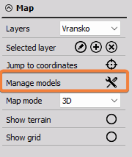
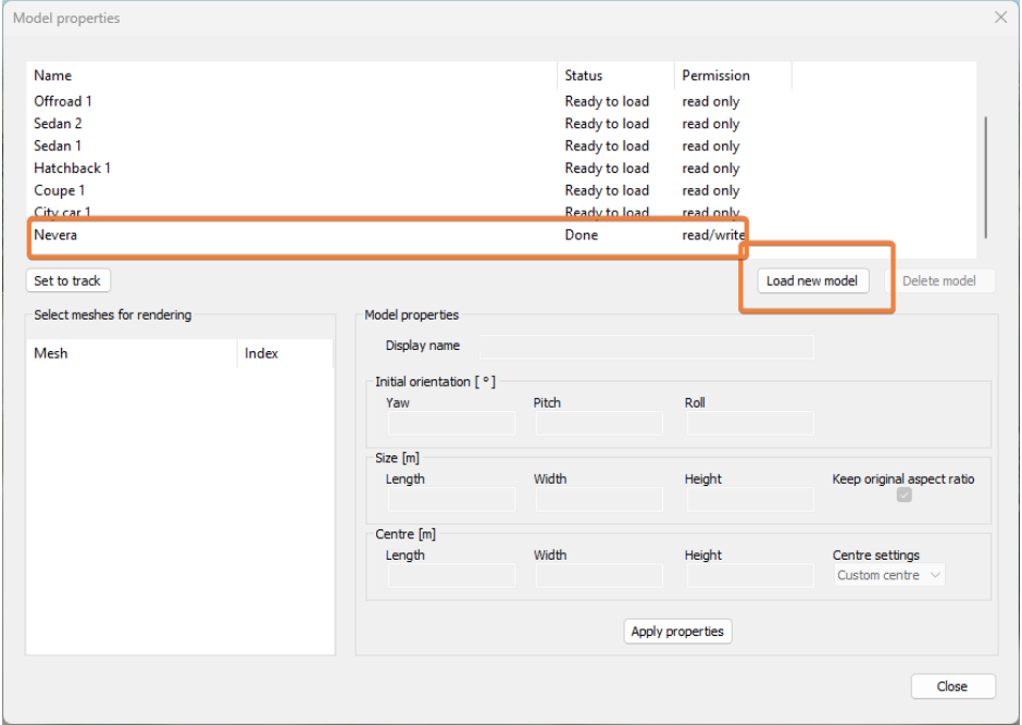
When the window opens, click ‘Load New Model’, and the Nevera model should load properly.

Once a model is loaded, you can define its size and center. You can check ‘Keep Original Aspect Ratio’ or define each dimension manually. In this case, set only the length to 4.75 m and define the center of the model as shown in the image below.

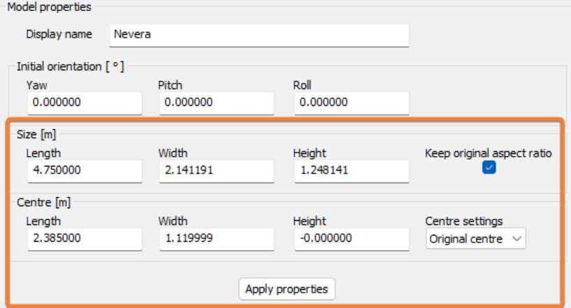
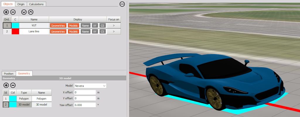
You can now select Nevera as a 3D model in Polygon to drive around the track.

Next, in the measurement screen, add an indicator lamp that will turn red if the calculated distance is less than 5 cm. Additionally, add another lamp for the Overlap calculation.

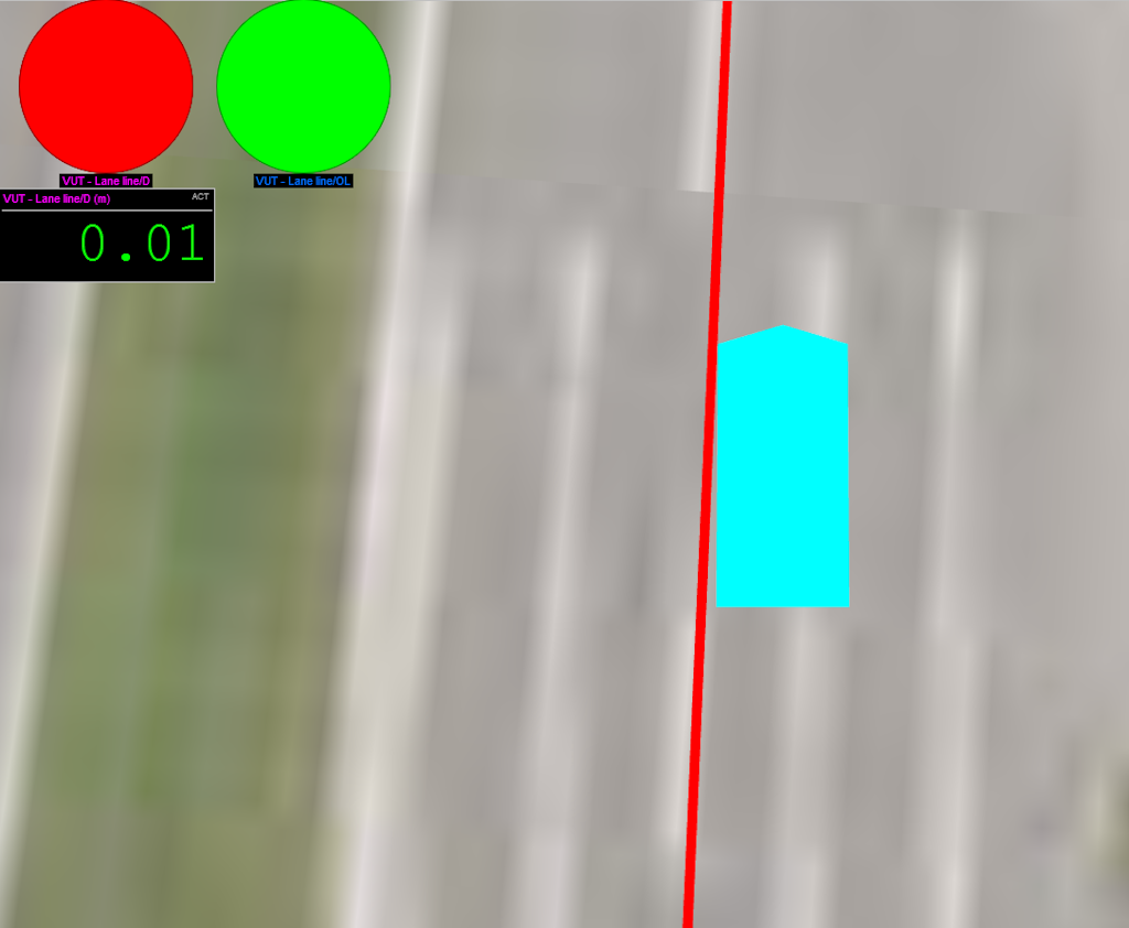
With this setup, you can perform the Lane Assist Test and monitor the distance between the VUT and the lane. In a real measurement, you can also add a camera and/or microphone, in combination with positioning data, to monitor the system’s functionality.
Page 1 of 15